Program Logics for Homogeneous Meta-Programming

1 Introduction

Meta-programming is the generation or manipulation of programs, or parts of programs, by other programs, i.e. in an algorithmic way. Meta-programming is commonplace, as evidenced by the following examples: compilers, compiler generators, domain specific language hosting, extraction of programs from formal specifications, and refactoring tools.

Many programming languages, going back at least as far as Lisp, have explicit meta-programming features. These can be classified in various ways such as: generative (program creation), intensional (program analysis), compile-time (happening while programs are compiled), run-time (taking place as part of program execution), heterogeneous (where the system generating or analysing the program is different from the system being generated or analysed), homogeneous (where the systems involved are the same), and lexical (working on simple strings) or syntactical (working on abstract syntax trees). Arguably the most common form of meta-programming is reflection, supported by mainstream languages such as Java, C#, and Python. Web system languages such as PHP use meta-programming to produce web pages containing JavaScript; JavaScript (in common with some other languages) does meta-programming by dynamically generating strings and then executing them using its eval function. In short, meta-programming is a mainstream activity.

An important type of meta-programming is generative meta-programming, specifically homogeneous meta-programming. The first language to support homogeneous meta-programming was Lisp with its S-expression based macros; Scheme’s macros improve upon Lisp’s by being fully hygienic, but are conceptually similar. Perhaps unfortunately, the power of Lisp-based macros was long seen to rest largely on Lisp’s minimalistic syntax; it was not until MetaML [17] that a modern, syntactically rich language was shown to be capable of homogeneous meta-programming. Since then, MetaOCaml [18] (a descendant of MetaML), Template Haskell [16] (a pure compile-time meta-programming language) and Converge [19] (inspired by Template Haskell and adding features for embedding domain specific languages) have shown that a variety of modern programming languages can house homogeneous generative meta-programming, and that this allows powerful, safe programming of a type previously impractical or impossible.

Meta-Programming & Verification. The ubiquity of meta-programming demonstrates its importance; by extension, it means that the correctness of much modern software depends on the correct use of meta-programming. Surprisingly, correctness and meta-programming have received little joint attention. In particular, there seem to be no program logics for meta-programming languages, homogeneous or otherwise. We believe that the following reasons might be partly responsible.

• First, developing logics for non-meta-programming programming languages is already a hard problem, and only recently have satisfactory solutions been found for reasoning about programs with higher-order functions, state, pointers, continuations or concurrency [1, 14, 21]. Since reasoning about meta-programs contains reasoning about normal programs as a special case, program logics for meta-programming are at least as complicated as logics for normal languages.
• Second, it is often possible to side-step the question of meta-programming correctness altogether by considering only the final product of meta-programming. Compilation is an example where the meta-programming machinery is typically much more complex than the end product. Verifying only the output of a meta-programming process is inherently limited, because knowledge garnered from the input to the process cannot be used.
• Finally, static typing of meta-programming is challenging, and still not a fully solved problem. Consequently, most meta-programming languages are at least partly dynamically typed (including MetaOCaml); Template Haskell on the other hand intertwines code generation with type-checking in complicated ways. Logics for such languages are not well understood in the absence of other meta-programming features; moreover, many meta-programming languages have additional features such as capturing substitution, pattern matching of code, and splicing of types, which are largely unexplored theoretically. Heterogeneous meta-programming adds the complication of multi-language verification.

Contributions. The present paper is the first in a series investigating the use of program logics for the specification and verification of meta-programming. The aim of the series is to unify and relate all key meta-programming concepts using program logics. One of our goals is to achieve coherency between existing logics for programming languages and their meta-programming extensions (i.e. the former should be special cases of the latter). The contributions of this paper are as follows (all proofs have been omitted in the interests of brevity; they can be found in [4]):

• We provide the first program logic for a generative, homogeneous meta-programming language (Pcfdp, a variant of Davies and Pfenning’s MiniML_e^□ [6], itself an extension of Pcf [8]). The logic smoothly generalises previous work on axiomatic semantics for the ML family of languages [1, 2, 9, 11, 12, 21]. The logic is for total correctness (for partial correctness see [4]). A key feature of our logic is that for Pcfdp programs that don’t do meta-programming, i.e. programs in the Pcf-fragment, reasoning can be done in the simpler logic [9, 11] for Pcf. Hence reasoning about meta-programming does not impose an additional burden on reasoning about normal programs.
• We show that our logic is relatively complete in the sense of Cook [5] (Section 5).
• We demonstrate that the axiomatic semantics induced by our logic coincides precisely with the contextual semantics given by the reduction rules of Pcfdp (Section 5).
• We present an additional inference system for characteristic formulae which enables, for each program M, the inductive derivation of a pair A,B of formulae which describe completely M’s behaviour (descriptive completeness [10], Section 5).

2 The Language

This section introduces Pcfdp, the homogeneous meta-programming language that is the basis of our study. Pcfdp is a meta-programming variant of call-by-value (CBV) Pcf [8], extended with the meta-programming features of Mini-ML_e^□[6, Section 3]. From now on we will simply speak of Pcf to mean CBV Pcf. Mini-ML_e^□ was the first typed homogeneous meta-programming language to provide a facility for executing generated code. Typing the execution of generated code is a difficult problem. Mini-ML_e^□ achieves type-safety with two substantial restrictions:

• Only closed generated code can be executed.
• Variables free in code cannot be λ-abstracted or be recursion variables.

Mini-ML_e^□ was one of the first meta-programming languages with a Curry-Howard correspondence, although this paper does not investigate the connection between program logic and the Curry-Howard correspondence. Pcfdp is essentially Mini-ML_e^□, but with a slightly different form of recursion that can be given a moderately simpler logical characterisation. Pcfdp is an ideal vehicle for our investigation for two reasons. First, it is designed to be a simple, yet non-trivial meta-programming language, having all key features of homogeneous generative meta-programming while removing much of the complexity of real-world languages (for example, Pcfdp’s operational semantics is substantially simpler than that of the MetaML family of languages [17]). Second, it is built on top of Pcf, a well-understood idealised programming language with existing program logics [9, 11], which means that we can compare reasoning in the Pcf-fragment with reasoning in full Pcfdp.

Pcfdp extends Pcf with one new type ⟨α⟩ as well as two new term constructors, quasi-quotes ⟨M⟩ and an unquote mechanism let ⟨x⟩ = M in N. Quasi-quotes ⟨M⟩ represent the code of M, and allow code fragments to be simply expressed in normal concrete syntax; quasi-quotes also provide additional benefits such as ensuring hygiene. The quasi-quotes we use in this paper are subtly different from the abstract syntax trees (ASTs) used in languages like Template Haskell and Converge. In such languages, ASTs are a distinct data type, shadowing the conventional language feature hierarchy. In this paper, if M has type α, then ⟨M⟩ is typed ⟨α⟩. For example, ⟨1+7⟩ is the code of the program 1+7 of type ⟨Int⟩. ⟨M⟩ is a value for all M and hence ⟨1+7⟩ does not reduce to ⟨8⟩. Extracting code from a quasi-quote is the purpose of the unquote let ⟨x⟩ = M in N. It evaluates M to code ⟨M′⟩, extracts M′ from the quasi-quote, names it x and makes M′ available in N without reducing M′. For example

first reduces the application to ⟨1+7⟩, then extracts the code from ⟨1+7⟩, names it x and makes it available unevaluated to the code ⟨λn.xⁿ⟩:

Fig. 1: Key typing rules for Pcfdp.

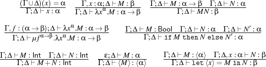
Not evaluating code after extraction from a quasi-quote is fundamental to meta-programming because it enables the construction of code other than values under λ-abstractions. This is different from the usual reduction strategies of CBV-calculi — Section 6 discusses briefly how Pcfdp might nevertheless be embeddable into Pcf. Unquote can also be used to run a meta-program: if M evaluates to a quasi-quote ⟨N⟩, the program let ⟨x⟩ = M in x evaluates M, extracts N, binds N to x and then runs x, i.e. N. In this sense, Pcfdp’s unquote mechanism unifies splicing and executing quasi-quoted code, where the MetaML family of languages uses different primitives for these two functions [17].

Syntax and Types. We now formalise Pcfdp’s syntax and semantics, assuming a set of variables, ranged over by x,y,f,u,m,... (for more details see [6, 8]).

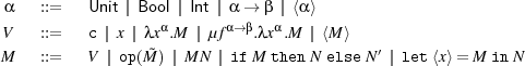
Here α ranges over types, V over values and M ranges over programs. Constants c range over the integers 0,1,-1,..., booleans t,f, and () of type Unit, op ranges over the usual first-order operators like addition, multiplication, equality, conjunction, negation, comparison, etc., with the restriction that equality is not defined on expressions of function type or of type ⟨α⟩. The recursion operator is μf.λx.M. The free variables fv(M) of M are defined as usual with two new clauses: fv(⟨M⟩)fv(M) and fv(let ⟨x⟩ = M in N)fv(M)∪(fv(N)\{x}). We write λ().M for λx^Unit.M and let x = M in N for (λx.N)M, assuming that xfv(M) in both cases. A typing environment (Γ,Δ,...) is a finite map x₁ : α₁,...,x_k : α_k from variables to types. The domain dom(Γ) of Γ is the set {x₁,...,x_n}, assuming that Γ is x₁ : α₁,...,x_n : α_n. We also write ϵ for the empty environment. The typing judgement is written Γ;Δ ⊢ M : α where we assume that dom(Γ)∩dom(Δ) = ∅. We write ⊢ M : α for ϵ;ϵ ⊢ M : α. We say a term M is closed if ⊢ M : α. We call Δ a modal context in Γ;Δ ⊢ M : α. We say a variable x is modal in Γ;Δ ⊢ M : α if x ∈dom(Δ). Modal variables represent code inside other code, and code to be run. The key type-checking rules are given in Figure 1. Typing for constants and first-order operations is standard.

Noteworthy features of the typing system are that modal variables cannot be λ- or μ-abstracted, that all free variables in quasi-quotes must be modal, and that modal variables can only be generated by unquotes. [6] gives detailed explanations of this typing system and its relationship to modal logics.

The reduction relation → is unchanged from Pcf for the Pcf-fragment of Pcfdp, and adapted to Pcfdp as follows. First we define define reduction contexts, by extending those for Pcf as follows.

Now → is defined as usual on closed terms with one new rule.

We write →→ for →^*. M ⇓ V means that M →→ V for some value V . We write M ⇓ if M ⇓ V for some appropriate V .

By ⊑_Γ;Δ;α (usually abbreviated to just ⊑) we denote the usual typed contextual preconguence: if Γ;Δ ⊢ M_i : α for i = 1,2 then: M₁ ⊑_Γ;Δ;αM₂ iff for all closing context C[⋅] such that ⊢ C[M_i] : Unit (i = 1,2) we have C[M₁] ⇓ implies C[M₂] ⇓. We write ≃ for ⊑∩⊑^-1 and call ≃ contextual congruence. Other forms of congruence are possible. Our choice means that code can only be observed contextually by running it. Hence for example ⟨M⟩ and ⟨λx.Mx⟩ are contextually indistinguishable if xfv(M), as are ⟨1+2⟩ and ⟨3⟩. This coheres well with the notion of equality in Pcf, and facilitates a smooth integration of the logics for Pcfdp with the logics for Pcf. Some meta-programming languages are more discriminating, allowing, e.g. printing of code, which can distinguish α-equivalent programs. It is unclear how to design logics for such languages.

Examples. We now present classic generative meta-programs in Pcfdp. We reason about some of these programs in later sections.

The first example is from [6] and shows how generative meta-programming can stage computation, which can be used for powerful domain-specific optimisations. As an example, consider staging an exponential function λna.aⁿ. It is generally more efficient to run λa.a×a×a than (λna.aⁿ) 3, because the recursion required in computing aⁿ for arbitrary n can be avoided. Thus if a program contains many applications (λna.aⁿ) 3, it makes sense to specialise such applications to λa.a×a×a. Meta-programming can be used to generate such specialised code as the following example shows.

This function has type ⊢power : Int →⟨Int →Int⟩. This type says that power takes an integer and returns code. That code, when run, is a function from integers to integers. More efficient specialisers are possible. This program can be used as follows.

The next example is lifting [6], which plays a vital role in meta-programming. Call a type α basic if it does not contain the function space constructor, i.e. if it has no subterms of the form β → β′. The purpose of lifting is to take an arbitrary value V of basic type α, and convert (lift) it to code ⟨V⟩ of type ⟨α⟩. Note that we cannot simply write λx.⟨x⟩ because modal variables (i.e. variables free in code) cannot be λ-abstracted. For α = Int the function is defined as follows:

Note that liftInt 3 evaluates to ⟨0+1+1+1⟩, not ⟨3⟩. In more expressive meta-programming languages such as Converge the corresponding program would evaluate to ⟨3⟩, which is more efficient, although ⟨0+1+1+1⟩ and ⟨3⟩ are observationally indistinguishable.

Lifting easily extended to Unit and Bool, but not to function types. For basic types ⟨α⟩ we can use the following definition:

Pcfdp can implement a function of type ⟨α⟩→ α for running code [6]:

3 A Logic for Total Correctness

This section defines the syntax and semantics of the logic. Our logic is a Hoare logic with pre- and post-conditions in the tradition of logics for ML-like languages [1, 2, 11, 12]. Expressions, ranged over by e,e′,... and formulae A,B,... of the logic are given by the grammar below, using the types and variables of Pcf.

The logical language is based on standard first-order logic with equality. Other quantifiers and propositional connectives like ⊃ (implication) are defined by de Morgan duality. Quantifiers range over values of appropriate type. Constants c and operations op are those of Section 2.

The proposed logic extends the logic for Pcf of [9, 10, 11] with a new code evaluation primitive u = ⟨m⟩{A}. It says that u, which must be of type ⟨α⟩, denotes (up to contextual congruence) a quasi-quoted program ⟨M⟩, such that whenever M is executed, it converges to a value; if that value is denoted by m then A makes a true statement about that value. We recall from [9, 10, 11] that u∙e = m{A} says that (assuming u has function type) u denotes a function, which, when fed with the value denoted by e, terminates and yields another value. If we name this latter value m, A holds. We call the variable m in u∙e = m{A} and u = ⟨m⟩{A} an anchor. The anchor is a bound variable with scope A. The free variables of e and A, written fv(e) and fv(A), respectively, are defined as usual noting that fv(u = ⟨m⟩{A})(fv(A)\{m})∪{u}. We use the following abbreviations: A^-x indicates that xfv(A) while e ⇓ means ∃x^α.e = x, assuming that e has type α. We let m = ⟨e⟩ be short for m = ⟨x⟩{x = e} where x is fresh, m∙e = e′ abbreviates m∙e = x{x = e′} where x is fresh. We often omit typing annotations in expressions and formulae.

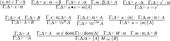
Judgements (for total correctness) are of the form {A} M :m {B}. The variable m is the anchor of the judgement, is a bound variable with scope B, and not modal. The judgement is to be understood as follows: if A holds, then M terminates to a value, and if we denote that value m, then B holds. If a variable x occurs freely in A or in B, but not in M, then x is an auxiliary variable of the judgement {A} M :m {B}. With environments as in Section 2, the typing judgements for expressions and formulae are Γ;Δ ⊢ e : α and Γ;Δ ⊢ A, respectively. The typing rules are given in Appendix A, together with the typing of judgements. The anchor in u = ⟨m⟩{A} is modal, while it is not modal in u∙e = m{A}.

The logic has the following noteworthy features. (1) Quantification is not directly available on modal variables. (2) Equality is possible between modal and non-modal variables. The restriction on quantification makes the logic weaker for modal variables than first-order logic. Note that if x is modal in A we can form ∀y.(x = y ⊃ A), using an equation between a modal and a non-modal variable. Quantification over all variables is easily defined by extending the grammar with a modal quantifier which ranges over arbitrary programs, not just values:

For ∀x□α.A to be well-formed, x must be modal and of type α in A. The existential modal quantifier is given by de Morgan duality. Modal quantification is used only in the metalogical results of Section 5. We sometimes drop type annotations in quantifiers, e.g. writing ∀x.A. This shorthand will never be used for modal quantifiers. We abbreviate modal quantification to ∀x□.A. From now on, we assume all occurring programs, expressions, formulae and judgements to be well-typed.

Examples of Assertions & Judgements. We continue with a few simple examples to motivate the use of our logic.

• The assertion m = ⟨3⟩, which is short for m = ⟨x⟩{x = 3} says that m denotes code which, when executed, will evaluate to 3. It can be used to assert on the program ⟨1+2⟩ as follows: {T} ⟨1+2⟩ :m {m = ⟨3⟩}
• Let Ω_α be a non-terminating program of type α (we usually drop the type subscript). When we quasi-quote Ω, the judgement {T} ⟨Ω⟩ :m {T} says (qua precondition) that ⟨Ω⟩ is a terminating program. Indeed, that is the strongest statement we can make about ⟨Ω⟩ in a logic for total correctness.
• The assertion ∀x^Int.m∙x = y{y = ⟨x⟩} says that m denotes a terminating function which receives an integer and returns code which evaluates to that integer. Later we use this assertion when reasoning about liftInt which has the following specification.

• The formula A_u∀n^Int ≥ 0.∃f^Int→Int.(u ∙ n = ⟨f⟩∧∀x^Int.f ∙ x = xⁿ) says that u denotes a function which receives an integer n as argument, to return code which when evaluated and fed another integer x, computes the power xⁿ, provided n≥ 0. We can show that {T} power :u {A_u} and {A_u} u 7 :r {r = ⟨f⟩{∀x.f ∙x = x⁷}}.
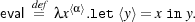
• The formula ∀x^⟨α⟩y^α.(x = ⟨y⟩⊃ u ∙ x = y) can be used to specify the evaluation function from Section 2: {T} eval :u {∀x^⟨α⟩y^α.(x = ⟨y⟩⊃ u∙x = y)}

Models and the Satisfaction Relation. This section formally presents the semantics of our logic. We begin with the notion of model. The key difference from the models of [11] is that modal variables denote possibly non-terminating programs.

Fig. 2: Key total correctness axioms for Pcfdp.

Let Γ,Δ be two contexts with disjoint domains (the idea is that Δ is modal while Γ is not). A model of type Γ;Δ is a pair (ξ,σ) where ξ is a map from dom(Γ) to closed values such that ⊢ ξ(x) : Γ(x); σ is a map from dom(Δ) to closed programs ⊢ σ(x) : Δ(x). We also write (ξ,σ)^Γ;Δ to indicate that (ξ,σ) is a model of type Γ;Δ. We write ξ⋅x : V for ξ∪{(x,V )} assuming that xdom(ξ), and likewise for σ⋅x : VM. We can now present the semantics of expressions. Let Γ;Δ ⊢ e : α and assume that (ξ,σ) is a Γ;Δ-model, we define [[e]]_(ξ,σ) by the following inductive clauses. [[c]]_(ξ,σ)c, [[op(ẽ)]]_(ξ,σ)op([[ẽ]]_(ξ,σ)), [[x]]_(ξ,σ)(ξ∪σ)(x). The satisfaction relation for formulae has the following shape. Let Γ;Δ ⊢ A and assume that (ξ,σ) is a Γ;Δ-model. We define (ξ,σ)A as usual with two extensions.

• (ξ,σ)e = e′ iff [[e]]_(ξ,σ) ≃ [[e′]]_(ξ,σ).
• (ξ,σ)¬A iff (ξ,σ) ⁄A.
• (ξ,σ)A∧B iff (ξ,σ)A and (ξ,σ)B.
• (ξ,σ)∀x^α.A iff for all closed values V of type α: (ξ⋅x : V,σ)A.
• (ξ,σ)u∙e = x{A} iff ([[u]]_(ξ,σ)[[e]]_(ξ,σ)) ⇓ V and (ξ⋅x : V,σ)A.
• (ξ,σ)u = ⟨m⟩{A} iff [[u]]_(ξ,σ) ⇓⟨M⟩, M ⇓ V and (ξ,σ⋅m : V )A.

To define the semantics of judgements, we need to say what it means to apply a model (ξ,σ) to a program M, written M(ξ,σ). That is defined as usual, e.g. x(ξ,σ)(ξ∪σ)(x) and (MN)(ξ,σ)M(ξ,σ)N(ξ,σ).

The satisfaction relation {A} M :m {B} is given next. Let Γ;Δ;α ⊢{A} M :m {B}. Then

This is the standard notion of total correctness, adapted to the present logic.

Fig. 3: Key Pcfdp inference rules for total correctness.

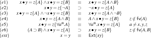
Axioms. This section introduces the key axioms of the logic. All axioms of [9, 10, 11] remain valid. We add axioms for x = ⟨y⟩{A}. Tacitly, we assume typability of all axioms. Some key axioms are given in Figure 2, more precisely, the axioms are the universal closure of the formulae presented in Figure 2. The presentation of axioms uses the following abbreviation: Extq(xy) stands for ∀a.(x = ⟨z⟩{z = a}≡ y = ⟨z⟩{z = a}).

Axiom (q1) says that if the quasi-quote denoted by x makes A true (assuming the program in that quasi-quote is denoted by y), and in the same way makes B true, then it also makes A∧B true, and vice versa. Axiom (q2) says that if the quasi-quote denoted by x contains a terminating program, denoted by y, and makes ¬A true, then it cannot be the case that under the same conditions A holds. The reverse implication is false, because ¬x = ⟨y⟩{A} is also true when x denotes a quasi-quote whose contained program is diverging. Next is (q3): x = ⟨y⟩{A} says in particular that x denotes a quasi-quote containing a terminating program, so ¬x = ⟨y⟩{B} can only be true because B is false. Axioms (q4,q5) let us move formulae and quantifiers in and out of code-evaluation formulae, as long as the anchor is not inappropriately affected. Axiom (q6) enables us to weaken a code-evaluation formula. The code-extensionality axiom (ext_q) formalises what it means for two quasi-quotes to be equal: they must contain observationally indistinguishable code.

Rules. Key rules of inference can be found in Figure 3. We write ⊢{A} M :m {B} to indicate that {A} M :m {B} is derivable using these rules. Rules make use of capture-free syntactic substitutions e[e′∕x], A[e∕x] which is straightforward, except that in e[e′∕x] and A[e∕x], x must be non-modal. Structural rules like Hoare’s rule of consequence, are unchanged from [9, 10, 11] and used without further comment. The rules in Figure 3 are standard and also unchanged from [9, 10, 11] with three significant exceptions, explained next.

[Var] adds x ⇓, i.e. ∃a.x = a in the precondition. By construction of our models,x ⇓ is trivially true if x is non-modal. If x is modal, the situation is different because x may denote a non-terminating program. In this case x ⇓ constrains x so that it really denotes a value, as is required in a total correctness logic.

[Quote] says that ⟨M⟩ always terminates (because the conclusion’s precondition is simply T). Moreover, if u denotes the result of evaluating ⟨M⟩, i.e. ⟨M⟩ itself, then, assuming A holds (i.e., given the premise, if M terminates), u contains a terminating program, denoted m, making B true. Clearly, in a logic of total correctness, if M is not a terminating program, A will be equivalent to F, in which case, [Quote] does not make a non-trivial assertion about ⟨M⟩ beyond stating that ⟨M⟩ terminates.

[Unquote] is similar to the usual rule for let x = M in N which is easily derivable:

Rules for let ⟨x⟩ = M in N are more difficult because a quasi-quote always terminates, but the code it contains may not. Moreover, even if M evaluates to a quasi-quote containing a divergent program, the overall expression may still terminate, because N uses the destructed quasi-quote in a certain manner. Here is an example:

[Unquote] deals with this complication in the following way. Assume {A} M :m {B ⊃ m = ⟨x⟩{C}} holds. If M evaluates to a quasi-quote containing a divergent program, B would be equivalent to F. The rule uses B ⊃ C in the right premise, where x is now a free variable, hence also constrained by C. If B is equivalent to F, the right precondition is T, i.e. contains no information, and M’s termination behaviour cannot depend on x, i.e. N must use whatever x denotes in a way that makes the termination or otherwise of N independent of x. Apart from this complication, the rule is similar to [Let].

4 Reasoning Examples

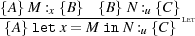
We now put our logic to use by reasoning about some of the programs introduced in Section 2. The derivations use the abbreviations of Section 3 and omit many steps that are not to do with meta-programming. Several reduction steps are justified by the following two standard structural rules omitted from Figure 3.

Example 1. We begin with the simple program {T} ⟨1+2⟩ :m {m = ⟨3⟩}. The derivation is straightforward.

Example 2. This example deals with the code of a non-terminating program. We derive {T} ⟨Ω⟩ :m {T}. This is the strongest total correctness assertion about ⟨Ω⟩. In the proof, we assume that {F} Ω :a {T} is derivable, which is easy to show.

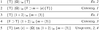
Example 3. The third example destructs a quasi-quote and then injects the resulting program into another quasi-quote.

We derive the assertion in small steps to demonstrate how to apply our logical rules.

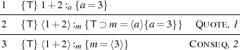
Example 4. Now we show that destructing a quasi-quote containing a non-terminating program, and then not using that program still leads to a terminating program. This reflects the operational semantics in Section 2.

The derivation follows.

The examples below make use of the following convenient forms of the recursion rule and [Unquote]. Both are easily derived.

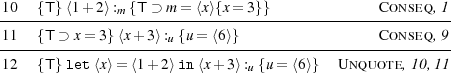
Example 5. This example extract a non-terminating program from a quasi-quote, and injects it into a new quasi-quote. Our total-correctness logic cannot say anything non-trivial about the resulting quasi-quote (cf. Example 2):

The derivation is straightforward.

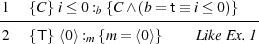
Example 6. Now we reason about liftInt from Section 3. In the proof we assume that i,n range over non-negative integers. Let A_n^uu∙n = m{m = ⟨n⟩}. We are going to establish the following assertion from Section 3: {T} liftInt :u {∀n.A_n^u}. We set Ci ≤ n∧∀j < n.A_j^g, Di > 0∧∀r.(0 ≤ r < n ⊃ g∙r = m{m = ⟨r⟩}) and Plet ⟨x⟩ = g(i-1) in ⟨x+1⟩.

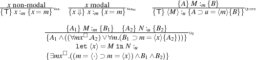
Example 7. We close this section by reasoning about the staged power function from Section 2. Assuming that i,j,k,n range over non-negative integers, we define B_n^uu∙n = m{m = ⟨y⟩{∀j.y∙j = jⁿ}}. In the derivation, we provide less detail than in previous proofs for readability.

5 Completeness

This section answers three important metalogical questions about the logic for total correctness introduced in Section 3.

• Is the logic relatively complete in the sense of Cook [5]? This question asks if {A} M :m {B} implies ⊢{A} M :m {B} for all appropriate A,B. Relative completeness means that the logic can syntactically derive all semantically true assertions, and reasoning about programs does not need to concern itself with models. We can always rely on just syntactic rules to derive an assertion (assuming an oracle for Peano arithmetic).

  ---

  

  
  

  Fig. 4: Key inference system for TCAPs, where m = ⟨⋅⟩ is short for m = ⟨z⟩{T}.

  ---

• Is the logic observationally complete [10]? The second question investigates if the program logic makes the same distinctions as the observational congruence. In other words, does M ≃ N hold iff for all suitably typed A,B: {A} M :m {B} iff {A} N :m {B}? Observational completeness means that the operational semantics (given by the contextual congruence) and the axiomatic semantics given by logic cohere with each other.
• If a logic is observationally complete, we may ask: given a program M, can we find, by induction on the syntax of M, characteristic formulae A,B such that (1) {A} M :m {B} and (2) for all programs N: M ≃ N iff {A} N :m {B}? If characteristic formulae always exist, the semantics of each program can be obtained and expressed finitely in the logic, and we call the logic descriptively complete [10].

Following [3, 10, 21], we answer all questions in the affirmative.

Characteristic Formulae. Program logics reason about program properties denoted by pairs of formulae. But what are program properties? We cannot simply say program properties are subsets of programs, because there are uncountably many such subsets, yet only countably many pairs of formulae. To obtain a notion of program property that is appropriate for a logic of total correctness, we note that such logics cannot express that a program diverges. More generally, if {A} M :m {B} and M ⊑ N (where ⊑ is the contextual pre-congruence from Section 2), then also {A} N :m {B}. Thus pairs A,B talk about upwards-closed sets of programs. A set S of programs is upwards-closed if M ∈ S and M ⊑ N together imply that N ∈ S. It can be shown that each upwards closed set of Pcfdp-terms has a unique least element up-to ≃. Thus each upwards-closed set has a distinguished member, is its least element. Consequently a pair A,B is a characteristic assertion pair for M (at m) if M is the least program w.r.t. ⊑ such that {A} M :m {B}, leading to the following key definition.

Definition. A pair (A,B) is a total characteristic assertion pair, or TCAP, of M at u, if the following conditions hold (in each clause we assume well-typedness).

1. (soundness) {A} M :u {B}.
2. (MTC, minimal terminating condition) For all models (ξ,σ), M(ξ,σ) ⇓ if and only if (ξ,σ)A.
3. (closure)  If {E} N :u {B} and E ⊃ A, then for all (ξ,σ): (ξ,σ)E implies M(ξ,σ) ⊑ N(ξ,σ).

A TCAP of M denotes a set of programs whose minimum element is M, and in that sense characterises that behaviour uniquely up to ⊑.

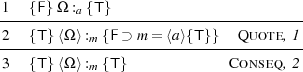
Descriptive Completeness. The main tool in answering the three questions posed above is the inference system for TCAPs, of which the key rules are given in Figure 4. The remaining rules are unchanged from [10]. We write ⊢tcap {A} M :u {B} to indicate that {A} M :u {B} is derivable in that new inference system. It is obvious that TCAPs can be derived mechanically from programs – no invariants for recursion have to be supplied manually.

The premise of [Unquote] in Figure 4 uses modal quantification. This is the only use of the modal quantifier. The semantics is: (ξ,σ)∀x□α.A iff for all closed programs M of type α: (ξ,σ⋅x : M)A. Syntactic reasoning with modal quantifiers needs a few straightforward quantifier axioms beyond those of first-order logic and those of Figure 2, for example ¬∀x□.x ⇓, and ¬∀x□.¬x ⇓. An interesting open question is whether modal quantification can be avoided altogether in constructing TCAPs.

Theorem 1.

1. (descriptive completeness for total correctness)  Assume Γ;Δ ⊢ M : α. Then ⊢tcap {A} M :u {B} implies (A,B) is a TCAP of M at u.
2. (observational completeness) M ≃ N if and only if, for each A and B, we have {A} M :u {B} iff {A} N :u {B}.
3. (relative completeness) Let B be upward-closed at u. Then {A} M :u {B} implies ⊢{A} M :u {B}.

6 Conclusion

We have proposed the first program logic for a meta-programming language, and established key metalogical properties like completeness and the correspondence between axiomatic and operational semantics. We are not aware of previous work on program logics for meta-programming. Instead, typing systems for statically enforcing program properties have been investigated. We discuss the two systems with the most expressive typing systems, Ωmega [15] and Concoqtion [7]. Both use indexed typed to achieve expressivity. Ωmega is a CBV variant of Haskell with generalised algebraic datatypes (GADTs) and an extensible kind system. In Ωmega, GADTs can express easily datatypes representing object-programs, whose meta-level types encode the object-level types of the programs represented. Tagless interpreters can directly be expressed and typed for these object programs. Ωmega is expressive enough to encode the MetaML typing system together with a MetaML interpreter in a type-safe manner. Concoqtion is an extension of MetaOCaml and uses the term language of the theorem prover Coq to define index types, specify index operations, represent the properties of indexes and construct proofs. Basing indices on Coq terms opens all mathematical insight available as Coq libraries to use in typing meta-programs. Types in both languages are not as expressive with respect to properties of meta-programs themselves, as our logics, which capture exactly the observable properties. Nevertheless, program logic and type-theory are not mutually exclusive; on the contrary, reconciling both in the context of meta-programming is an important open problem.

The construction of our logics as extensions of well-understood logics for Pcf indicates that logical treatment of meta-programming is mostly orthogonal to that of other language features. Hence [18] is an interesting target for generalising the techniques proposed here because it forms the basis of MetaOCaml, the most widely studied meta-programming language in the MetaML tradition. Pcfdp and [18] are similar as meta-programming languages with the exception that the latter’s typing system is substantially more permissive: even limited forms evaluation of open code is possible. We believe that a logical account of meta-programming with open code is a key challenge in bringing program logics to realistic meta-programming languages. A different challenge is to add state to Pcfdp and extend the corresponding logics. We expect the logical treatment of state given in [2, 21] to extend smoothly to a meta-programming setting. The main issue is the question what typing system to use to type stateful meta-programming: the system used in MetaOCaml, based on [18], is unsound in the presence of state due to a form of scope extrusion. This problem is mitigated in MetaOCaml with dynamic type-checking. As an alternative to dynamic typing, the Java-like meta-programming language Mint [20] simply prohibits the sharing of state between different meta-programming stages, resulting in a statically sound typing system. We believe that both suggestions can be made to coexist with modern logics for higher-order state [2, 21], in the case of [20] easily so.

The relationship between Pcfdp and Pcf, its non-meta-programming core, is also worth investigating. Pfenning and Davies proposed an embedding ⌜⋅⌝ from Pcfdp into Pcf, whose main clauses are given next.

We believe that this embedding is fully-abstract, but proving full abstraction is non-trivial because translated Pcfdp-term have Pcf-inhabitants which are not translations of Pcfdp-terms (e.g. λx^Int→Int.λ().x). A full abstraction proof might be useful in constructing a logically fully abstract embedding of the logic presented here into the simpler logic for Pcf from [9, 11]. A logical full abstraction result [13] is an important step towards integrating logics for meta-programming with logics for the produced meta-programs.

In the light of this encoding one may ask why meta-programming languages are relevant at all: why not simply work with a non-meta-programming language and encodings?

• We believe that nice (i.e. fully abstract and compositional) encodings might exist for simple meta-programming languages like Pcfdp because Pcfdp lives at the low end of meta-programming expressivity. For even moderately more expressive languages like [18] no fully abstract encodings into simple λ-calculi are known.
• A second reason is to do with efficiency, one of the key reasons for using meta-programming: encodings are unlikely to be as efficient as proper meta-programming.
• Finally, programs written using powerful meta-programming primitives are more readable and hence more easily evolvable than equivalent programs written using encodings.

References

A Typing Rules for Expressions, Formulae and Assertions

The key typing rules for expressions, formulae and judgements are summarised in Figure 5 above.

Fig. 5: Typing rules for expressions, formulae and judgements. Rules for constants and first-order operations omitted.

References

1. M. Berger. Program Logics for Sequential Higher-Order Control. In Proc. FSEN, pages 194–211, 2009.
2. M. Berger, K. Honda, and N. Yoshida. A Logical Analysis of Aliasing in Imperative Higher-Order Functions. J. Funct. Program., 17(4-5):473–546, 2007.
3. M. Berger, K. Honda, and N. Yoshida. Completeness and logical full abstraction in modal logics for typed mobile processes. In Proc. ICALP, pages 99–111, 2008.
4. M. Berger and L. Tratt. Program Logics for Homogeneous Metaprogramming. Long version of the present paper, to appear.
5. S. A. Cook. Soundness and completeness of an axiom system for program verification. SIAM J. Comput., 7(1):70–90, 1978.
6. R. Davies and F. Pfenning. A modal analysis of staged computation. J. ACM, 48(3):555–604, 2001.
7. S. Fogarty, E. Pašalić, J. Siek, and W. Taha. Concoqtion: Indexed Types Now! In Proc. PEPM, pages 112–121, 2007.
8. C. A. Gunter. Semantics of Programming Languages. MIT Press, 1995.
9. K. Honda. From Process Logic to Program Logic. In ICFP’04, pages 163–174. ACM Press, 2004.
10. K. Honda, M. Berger, and N. Yoshida. Descriptive and Relative Completeness of Logics for Higher-Order Functions. In Proc. ICALP, pages 360–371, 2006.
11. K. Honda and N. Yoshida. A compositional logic for polymorphic higher-order functions. In Proc. PPDP, pages 191–202, 2004.
12. K. Honda, N. Yoshida, and M. Berger. An Observationally Complete Program Logic for Imperative Higher-Order Functions. In LICS’05, pages 270–279, 2005.
13. J. Longley and G. Plotkin. Logical Full Abstraction and PCF. In Tbilisi Symposium on Logic, Language and Information, CSLI, 1998.
14. J. C. Reynolds. Separation logic: a logic for shared mutable data structures. In Proc. LICS’02, pages 55–74, 2002.
15. T. Sheard and N. Linger. Programming in Ωmega. In Proc. Central European Functional Programming School, pages 158–227, 2007.
16. T. Sheard and S. Peyton Jones. Template meta-programming for Haskell. In Proc. Haskell Workshop, pages 1–16, 2002.
17. W. Taha. Multi-Stage Programming: Its Theory and Applications. PhD thesis, Oregon Graduate Institute of Science and Technology, 1993.
18. W. Taha and M. F. Nielsen. Environment classifiers. In Proc. POPL, pages 26–37, 2003.
19. L. Tratt. Compile-time meta-programming in a dynamically typed OO language. In Proc. DLS, pages 49–64, Oct. 2005.
20. E. Westbrook, M. Ricken, J. Inoue, Y. Yao, T. Abdelatif, and W. Taha. Mint: Java multi-stage programming using weak separability. In Proc. PLDI, 2010. To appear.
21. N. Yoshida, K. Honda, and M. Berger. Logical reasoning for higher-order functions with local state. In Proc. Fossacs, LNCS, pages 361–377, 2007.