Also available as: PDF.
Storage strategies for collections in dynamically typed languages
| Carl Friedrich Bolz | Lukas Diekmann | Laurence Tratt |
| University of Düsseldorf | University of Düsseldorf | King's College London |
| Hasso Plattner Institute Potsdam | King's College London | |
| King's College London | ||
| http://cfbolz.de/ | http://lukasdiekmann.com/ | http://tratt.net/laurie/ |
Abstract
Dynamically typed language implementations often use more
memory and execute slower than their statically typed cousins,
in part because operations on collections of elements are
unoptimised. This paper describes storage strategies, which
dynamically optimise collections whose elements are instances
of the same primitive type. We implement storage strategies in
the PyPy virtual machine, giving a performance increase of 18%
on wide-ranging benchmarks of real Python programs. We show
that storage strategies are simple to implement, needing only
1500LoC in PyPy, and have applicability to a wide range of
virtual machines.
1. Introduction
Implemented naively, dynamically typed languages tend to have poor performance relative to statically typed languages [35]. The flexibility and dynamism of dynamically typed languages frustrates most traditional static optimisations. Just-In-Time (JIT) compilers defer optimisations until run-time, when the types of objects at specific points in a program can be identified, and specialised code can be generated. In particular, variables which reference common types such as integers can be ‘unboxed’ [8 , 24]: rather than being references to an object in the heap, they are stored directly where they are used. This lowers memory consumption, improves cache locality, and reduces the overhead on the garbage collector. Unboxing is an important technique in optimising such languages.
However, JITs do not directly influence how objects are laid out in the heap. Therefore as soon as objects are added to a collection (e.g. lists, dictionaries), virtual machines (VMs) such as PyPy have to revert to boxing objects. This is necessary since collections in dynamically typed languages can store objects of multiple types. We call collections which do so heterogeneously typed. Pointer tagging [21] – where the spare bits in an aligned pointer are used to represent primitive data-types such as integers – can partially alleviate this issue. However, tagging has few bits to play with and some primitive types (e.g. strings) are not easily tagged. Furthermore, tagging is complex to implement, and has hard to predict performance trade-offs (e.g. due to branch prediction). For reasons such as this, VMs such as HotSpot and PyPy forego tagging.
Dynamically typed languages therefore pay a significant performance penalty for the possibility that collections may store heterogeneously typed elements, even for programs which create no such collections. Statically typed languages can determine efficient storage representations of collections storing elements of a primitive type based on a collection’s static types. The underlying aim of this work is to find a simple means of achieving a similar effect in dynamically typed languages. Ideally, we want an approach which is simpler to implement, understand, and debug than tagging, and which, unlike tagging, is generalisable to an arbitrary number of primitive types.
This paper presents storage strategies, a novel approach for optimising the representation of homogeneously typed collections (e.g. a list whose elements are all strings) in VMs for dynamically typed languages, even for those types that cannot sensibly be represented by pointer tagging. In essence, each collection has a single storage strategy, though the storage strategy may change throughout the collection’s lifetime. When elements are added to an empty collection, and when those elements are homogeneously typed, an optimised storage strategy is used for the collection. When collections are heterogeneously typed, or when an optimised storage strategy is not available, a ‘fallback’ storage strategy is used, which works as a traditional dynamically typed VM does. Similarly, if an element of a different type is added to a previously homogeneously typed collection – forcing the collection to type dehomogenise – the collection’s storage strategy is changed to a generic one, and its elements’ representation changed. Fortunately, and as is common in dynamically typed languages [9, 23, 31], this wide-ranging dynamicity is used infrequently in practise. Similarly, the storage strategy is reset when a collection is emptied of elements. Though optimised storage strategies are free to operate as they please, they customarily unbox elements and store them alongside one another. Importantly, all this happens without any input from the end programmer and without observably changing behaviour.
In order to validate our approach, we modified the PyPy VM [32] with support for storage strategies. PyPy is a fully feature-compatible Python JITing VM [7], whose performance is amongst the best for dynamically typed VMs [6]. It therefore makes a good test platform for storage strategies since it is already fairly well optimised: as with any reasonably mature VM, meaningful optimisations become harder to find over time. As our experiments on real-world Python systems show, storage strategies are a powerful optimisation, increasing performance in our benchmarks by 18% and lowering peak memory usage by 6%. Because of this, storage strategies were merged into the PyPy development stream and have been part of shipping releases since version 1.9, released in June 2012. All the strategies we describe in this paper have been included in PyPy releases since then.
As our implementation shows, storage strategies also have the advantage of being lightweight: PyPy’s storage strategies are approximately 1500 LoC in total. In comparison to tagging, which must be spread throughout a VM, storage strategies are implemented in a single place and are more easily comprehended. Storage strategies can therefore be retrofitted to existing VMs, or used within execution engines running atop an existing VM (e.g. HotSpot). Furthermore, our experiments demonstrate that storage strategies are an orthogonal concept to tagging: we still get useful speedups of 12% on primitive types that are not amenable to tagging.
The paper is structured as follows. We first describe the general design of storage strategies (Section 3), before detailing the specific implementation of storage strategies in PyPy (Section 4). Using a wide range of benchmarks, we then evaluate the speed and memory utilisation of storage strategies in PyPy (Section 5). Our experimental system is fully repeatable and downloadable from http://soft-dev.org/pubs/files/storage_strategies/. This artefact was accepted by OOPSLA's artefact evaluation committee.
2. Background
2.1 Memory usage in dynamically typed languages
An implicit effect of dynamic typing is that every variable, object slot, and so on, can reference objects of arbitrary types. The most natural way to implement this is to box all objects: that is, to allocate them on the heap with a common header. Although objects of different types may have different (and differently sized) bodies, this allows a simple, common representation for all objects, which simplifies VM implementation considerably.
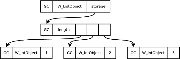
However, while universal boxing simplifies an implementation, it is inefficient. An integer in C typically occupies one word in memory; in PyPy, in contrast, 3 words are needed (1 word is reserved for the garbage collector; 1 word specifies the particular type of the object; and the final word stores the actual integer value). This problem is exacerbated when integers are stored in a list where the pointer to the boxed object adds further overhead. In PyPy, the seemingly simple list [1, 2, 3] is laid out in memory as in Figure 1.1 The raw memory statistics tell part of the story: a list of 1,000,000 integers takes 3.8MiB of memory in C but 15.3MiB in PyPy. However, other factors are important. In particular, boxed objects require memory on the heap to be allocated and later garbage collected, placing extra pressure on the garbage collector. Harder to quantify is the poor cache locality caused by the extra indirection of boxing, which may mean that sequentially accessed objects are spread around the heap.
One partial solution to this problem is pointer tagging [21]. This technique makes use of the fact that pointers to objects in a heap are aligned to multiples of 4 or 8 (depending on the combination of hardware and memory allocation library used). This means that at least 2 bits in every object pointer are unused, since they are always set to 0. Pointer tagging utilises these spare bits to differentiate genuine pointers from other sorts of information. Most commonly, this technique is used to store fixed-width datatypes – most commonly integers – into a single word. For example, any tagged pointer which has its least significant bit set may be defined to be a pointer – a simple AND can recover the real pointer address – otherwise it is an integer. In so doing, integers that fit into a machine word do not need to be allocated on the heap. Pointer tagging can allow a dynamically typed language to represent a list of integers as memory efficiently as C, substantially improving performance.
Pointer tagging is not without costs, however. Most obviously, every access of a tagged pointer requires a check of its tag type, and, in general, a modification to remove the tag and recover the pure value, hurting performance (not to mention occasional poor interaction with modern CPU’s branch prediction). As pointer accesses are extremely frequent, and spread throughout a VM, it is impossible to localise pointer tagging to a single portion of a VM: the complexity must be spread throughout the VM. Retrospective changes to pointer tagging involve widespread disruption to a VM; similarly, retrospectively introducing tagging into a previously non-tagging VM is likely to be a gargantuan effort. There are also only a finite number of spare bits in a pointer, putting a fixed, low, bound on the number of types that can be tagged. Finally, variable length data such as strings can not, in general, be tagged. Perhaps because of these reasons, pointer tagging is far from universal, and notable VMs such as the JVM’s HotSpot do not use this technique, as far as we are aware.
2.2 PyPy and tracing JITs
PyPy2 is a Python VM that is fully compatible with the ‘standard’ C Python VM3 (known as ‘CPython’). PyPy is written as an interpreter in RPython, a statically typed subset of Python that allows translation to (efficient) C. RPython is not a thin skin over C: it is fully garbage collected and contains several high-level data-types. More interestingly, RPython automatically generates a tracing JIT customised to the interpreter. Tracing JITs were initially explored by the Dynamo Project [3] and shown to be a relatively easy way to implement JITs [18]. The assumption underlying tracing JITs is that programs typically spend most of their time in loops and that these loops are very likely to take the same branches on each execution. When a ‘hot’ loop is detected at run-time, RPython starts tracing the interpreter (‘meta-tracing’), logging its actions [7]. When the loop is finished, the trace is heavily optimised and converted into machine code. Subsequent executions of the loop then use the machine code version.
An important property of tracing systems is that traces naturally lead to type specialisation, and escape analysis on the traces allows many actions on primitive types to be unboxed [8]. Specifically, most interpreters are able to be written in a style that makes unboxing primitive types stored in variables possible [6].
Meta-tracing allows fairly high performance VMs to be created with significantly less effort than traditional approaches [6]. PyPy is, on average, around 5–6 times faster on real-world benchmarks compared to CPython; it is even faster when measured against Jython, the Python implementation running atop the JVM [6]. In short, meta-tracing evens out the performance playing field for hard to optimise languages like Python.
3. Storage strategies
In Section 2.1, we saw how memory is typically used in dynamically typed languages. Pointer tagging is one partial solution but, as was noted, has limitations and costs as well. The obvious question is: can one come up with an alternative scheme which works well in practice? Our starting assumption is that a significant weakness of VMs such as PyPy is their treatment of collections. By optimising the use of primitive types in collections, we have a realistic hope of broadly matching – and, in some cases, perhaps exceeding – pointer tagging, without having to deal with its complexity.
As is common in high-performance VMs, it is impossible to optimise all use cases all of the time. Instead, we need to determine what bottlenecks real-world programs cause and focus our attention there. Our hypotheses of how real-world dynamically typed programs use collections are as follows:
- H1 It is uncommon for a homogeneously typed collection storing objects of primitive types to later type dehomogenise.
- H2 When a previously homogeneously typed collection type dehomogenises, the transition happens after only a small number of elements have been added.
We validate these hypotheses in Section 5.6; for the time being, we take them as given. These hypotheses give a clear target when it comes to optimising collections: collections storing elements of a single primitive type. We must also bear in mind that the second hypothesis, in particular, is one of probabilities, not absolutes: even if type dehomogenisation is rare, it can happen, and the possibility must be catered for.
The design of our solution is straightforward. Each collection references a storage strategy and a storage area. All operations on the collection are handed over to the storage strategy, which also controls how data is laid out in the storage area. An arbitrary number of strategies can be provided to efficiently store objects of different types. Although a collection can only have one strategy at any point in time, its strategy can change over time. As the name may suggest, this idea is an implementation of the Strategy design pattern [19].
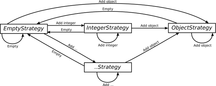
Figure 2 shows how a collection’s strategy can evolve over its lifetime. Collections start with the EmptyStrategy, which is a placeholder while the collection is empty; as soon as an object is put into the collection, a more specific strategy will be used. If an object of primitive type, such as an int, is added to the collection, and if an optimised strategy is available (e.g. IntegerStrategy), the collection switches to it; the strategy will unbox the element and store it. As more elements of that primitive type are added, the collection will grow accordingly. If an object of a different type is then added to the collection, the strategy will be changed to the ObjectStrategy, which has the same performance characteristics as a typical VM without storage strategies; any existing objects in the collection will have to be reboxed. Finally, if the collection is emptied of all objects, its strategy is returned to the EmptyStrategy.
Storage strategies have low overheads. Each collection needs only a single extra pointer to a strategy object. Each strategy can be a singleton or static class, allowing it to be shared between multiple collections, requiring a small, fixed overhead per process. As many strategies as desired can be implemented, and collections can easily move between strategies over their lifetime. Operations on collections need one extra method call on the strategy to be implemented, the cost of which should be offset by the time saved by not boxing as many elements.
4. Storage strategies in PyPy
4.1 Basic design
We have implemented storage strategies in PyPy for the three major forms of collections in Python – lists, sets, and dictionaries (known in different languages as maps or hashtables) – and three major primitive types – integers, floats, and strings. List and set storage strategies are relatively obvious; dictionaries, having both keys and values, less so. Although we could implement strategies for each pairwise (key, value) primitive type combination we believe this is unnecessary as the main bottleneck in dictionary performance is the hashing and comparing of keys. Therefore dictionary strategies dictate the storage of keys, but leave values boxed.
For each collection type X, we have implemented an EmptyXStrategy (for when the collection has no objects), an ObjectXStrategy (for storing objects of arbitrary types), and IntegerXStrategy, FloatXStrategy, and StringXStrategy (for the primitive types). Collections return to the EmptyXStrategy when their clear method is called. Since Python lists do not have such a method, they can not currently return to the EmptyListStrategy.
Each ObjectXStrategy largely reuses the relevant portion of pre-storage strategy code (with minor modifications), whereas the other strategies contain all-new code. In addition to the normal collection operations, we also added shortcuts to allow collections with optimised storage strategies to interact efficiently with each other (see Section 4.4 for further details). With the normal caution to readers about the dangers of over-interpreting Lines of Code (LoC) figures, the following details give a good idea of the simplicity of storage strategies. In total, storage strategies added 1500LoC4 to PyPy when merged in. Of that total, lists contribute 750LoC, sets 550, and dictionaries 200. The relatively small LoC count for dictionaries is due to the existing implementation of dictionaries already having storage strategy-like behaviour, which is hard to factor out from the newer, full-blown, storage strategies.
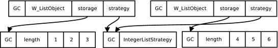
Figure 3 shows the memory layout of two lists using the IntegerListStrategy, one storing [1, 2, 3] and the other [4, 5, 6]. Comparing them to the conventional layout shown earlier in Figure 1, we can see that storage strategies unbox the integers, saving three words per element. Figure 3 also shows that the use of singleton strategies keeps the overhead of storage strategies to a fixed minimum.
As Figure 3 suggests, strategies add one extra word to each collection. If a program used a large number of small, almost exclusively, heterogeneously typed collections, the overhead of the extra word may outweigh the savings on homogeneously typed collections. Such behaviour seems unlikely, and none of our benchmarks exhibits it (see Section 5.6).
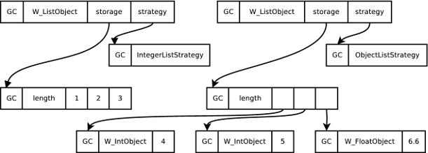
As motivated in Section 3, users of dynamically typed languages always have the possibility of changing an homogeneously typed collection into a heterogeneously typed collection: it is vital that storage strategies can cope with this. Figure 4 shows what happens when an object of a different type (in this case a float) is added to the previously homogeneously typed list of ints [4, 5, 6]. The integers in the list are (re)boxed, the list’s strategy is changed to the generic ObjectListStrategy, and the data section rewritten appropriately. Clearly, such reboxings are costly when applied to collections with large numbers of elements. Fortunately, this occurs relatively rarely in practise and when it does, collections contain only a single element on average (see Section 5.6). The disadvantages, therefore, are significantly outweighed by the advantages.
4.2 Implementation
2 def __init__(self):
3 self.strategy = EmptyListStrategy()
4 self.lstorage = None
5
6 def append(self, w_item):
7 self.strategy.append(self, w_item)
8
9 @singleton
10 class ListStrategy(object):
11 def append(self, w_list, w_item):
12 raise NotImplementedError("abstract")
13
14 @singleton
15 class EmptyListStrategy(ListStrategy):
16 def append(self, w_list, w_item):
17 if is_boxed_int(w_item):
18 w_list.strategy = IntegerListStrategy()
19 w_list.lstorage = new_empty_int_list()
20 elif ...:
21 ...
22 else:
23 w_list.strategy = ObjectListStrategy()
24 w_list.lstorage = new_empty_object_list()
25 w_list.append(w_item)
26
27 @singleton
28 class IntegerListStrategy(ListStrategy):
29 def append(self, w_list, w_item):
30 if is_boxed_int(w_item):
31 w_list.lstorage.append_int(unbox_int(w_item))
32 return
33 self.switch_to_object_strategy(w_list)
34 w_list.append(w_item)
35
36 def switch_to_object_strategy(self, w_list):
37 lstorage = new_empty_object_list()
38 for i in w_list.lstorage:
39 lstorage.append_obj(box_int(i))
40 w_list.strategy = ObjectListStrategy()
41 w_list.lstorage = lstorage
42
43 @singleton
44 class ObjectListStrategy(ListStrategy):
45 def append(self, w_list, w_item):
46 w_list.lstorage.append_obj(w_item)
To make our explanation of PyPy’s implementation of storage strategies somewhat more concrete, Figure 5 shows the relevant sections of code for the append method on lists. Although Figure 5 necessarily elides and simplifies various details, it gives a good flavour of the relative simplicity of storage strategies.
PyPy’s root object class is W_Object from which the list class W_ListObject inherits. Each instance of W_ListObject has a storage strategy and a storage area (which is controlled by the strategy). Calling append on a list object transfers control over to the list’s strategy (line 7): note that, as the first parameter, the storage strategy is passed a pointer to the list object so that it can, if necessary, change the storage strategy and / or storage area. All list storage strategies are singletons and subclasses of ListStrategy, which is an abstract class that can not be directly instantiated. Empty list objects therefore use a reference to the EmptyListStrategy class for their storage strategy.
When an object is appended to an empty list, the EmptyListStrategy first sees if an optimised storage strategy is available for that type of object (lines 17–21). For example, if the incoming object is an integer (line 17), IntegerListStrategy is used. If no optimised storage strategy is available, ObjectListStrategy is used as the fallback (lines 23–24). Once the new strategy is decided upon, its append method is then called (line 25).
The final interesting case is when appending an item to a list using an optimised storage strategy. For example, if the IntegerListStrategy is being used, then append has two choices. If the object being appended is also an integer (line 30), it is unboxed, added to the storage area, and the function returns (lines 31–32). If, however, an object of a different type is appended, the list must be switched to the ObjectListStrategy. First a temporary storage area is created (line 37), and all the list’s integers boxed and put into it (38–39). The temporary storage area then replaces the original and the strategy is updated (lines 40–41).
4.3 Exotic storage strategies
PyPy, as of writing, has 17 storage strategies, some of which implement less obvious optimisations.
For example, consider Python’s range(i, j, s) function which generates a list of integers from i to j in steps of s. Its most common uses are in for statements and functional idioms such as map. Conceptually, range creates a full list of integers, but this is highly inefficient in practise: its most common idioms of use require neither random access nor, often, do they even read the full list (e.g. when a for loop contains a break). In order to optimise this common idiom, Python 3’s range operator5 returns a special ‘range’ type which is not a proper list (for example, items can not be written to it). If the programmer does want to use it as a normal list, it must be manually converted.
Storage strategies provide a natural solution to this problem, optimising the common case, while making the general case transparent to the programmer. Internally, PyPy provides a RangeListStrategy, which the range function uses. A list using this strategy stores only three words of information, no matter the size of the range created: start, stop, and step (all as integers). Typical operations on such a collection (e.g. contains) do not need to search all elements, instead using a simple mathematical calculation. If the user does add or remove an element from the range, it changes to an appropriate strategy (e.g. IntegerListStrategy upon element removal). The beauty of storage strategies is that, outside the RangeListStrategy itself, only the range function needs to be aware of its existence. All other code operates on such collections in blissful ignorance. The implementation of RangeListStrategy is straightforward, being well under 200LoC, but leads to a highly effective optimisation.
Dictionaries have a special storage strategy IdentityDictStrategy which optimises the case where key equality and hashing are based on object identity. This happens when user-defined classes which inherit from Python’s root object class do not override equality and hashing. This allows operations on dictionaries storing such objects to be optimised more effectively.
Similarly, storage strategies can be used to provide versions of normal datatypes customised to specific use cases. Python modules, classes, and objects can all have their contents accessed as dictionaries. Modules’ and class’ dictionaries are rarely written to after initialization. Objects’ dictionaries, on the other hand, are often written to, but each class’s instances tends to have a uniform set of keys. Using maps [12] as inspiration, optimised storage strategies for objects, modules, and classes optimise these use cases [6]. A similar strategy is used for the dictionaries that hold the variadic arguments of functions that take arbitrary (keyword) arguments.
4.4 Optimising collection creation and initialisation
Conceptually, collections are always created with an EmptyXStrategy, with elements then added to them. In practice, PyPy has fast paths to optimise common cases which do not need the generality, and consequent overhead, associated with the simple route. We now give two examples.
First, collections are sometimes created where the type of all the elements is known in advance. A simple example is the split(d) method on strings, which separates a string (using d as a delimiter) into a list of sub-strings. Rather than create a collection which starts in the EmptyListStrategy before immediately transitioning to the StringListStrategy, a fast path allows lists to be created which are initialised to the StringListStrategy. This technique is particularly useful when PyPy knows that a collection will be homogeneously typed and can use an optimized strategy immediately. This bypasses type-checking every element of the new collection.
Second, collections are often initialised from another collection: for example, cloning a list, or initialising sets with lists. In Python, for example, it is common to initialise sets with lists i.e. set([1,3,2,2]) creates a set {1,2,3}. The naive approach to creating the set is to iterate over the list, boxing each of its elements if necessary, and then putting them into the set which – if it uses storage strategies – may then unbox them again. Since, in our implementation, the list will be stored using the IntegerListStrategy, a few LoC in the set initialization code can detect the use of the other collection’s strategy and access the integers directly. Not only does this bypass boxing, type-checking, and unboxing, it allows the set storage strategy to perform hash operations directly on the primitive types rather than requiring an expensive type dispatch.
4.5 Optimising type-based operations
Optimised storage strategies such as IntegerListStrategy can make use of the type of data to improve the efficiency of common operations. A simple example is the contains(o) method which returns true if o is found in a collection. The IntegerListStrategy has a specialised contains method which, if passed an integer, performs a fast machine word comparison with the collection’s contents. If passed a user object with a custom definition of equality, standard – expensive – method dispatch occurs. Since the most likely test of equality on a collection is to see if an object of the same type exists in it, this can be a substantial optimisation, and is only a few LoC long. Furthermore, it is a benefit even when the VM is running as a ‘pure’ interpreter (i.e. when the JIT is not running). This technique can be used for many other collection methods, such as a list’s sort or a set’s difference or issubset methods.
4.6 Interaction with RPython’s Tracing JIT
Storage strategies give PyPy extra information about the types of objects in a collection. Most obviously, when a collection uses an optimised storage strategy such as IntegerListStrategy, we implicitly know that every element in the collection must be an integer. This is of particular interest to RPython’s tracing JIT, which can use this knowledge to prove additional properties about a trace, leading to more extensive optimisation.
Consider the following code fragment:
for x in c:
i += x
Let us assume that c stores only integers. In a normal implementation, every read of an element from c would be followed by a type-check before the addition is performed, constituting a sizeable overhead in such a simple loop. With storage strategies, the first iteration of the list will deduce that the list uses the IntegerListStrategy. The resulting trace will naturally establish that the contents of c are not changed, and that since i is also an integer, no further type checks need to be performed on the elements coming out of c at all. No matter the size of the list, only a simple check on c’s strategy is needed before the loop is executed. Assuming this condition is met, the integers extracted from c can be accessed unboxed, leading to highly efficient machine code.
This same basic idea works equally well on more complex collection operations. Consider code which writes an object into a dictionary. Potentially, the object may provide custom hashing and comparison operations which may have arbitrary side effects, including mutating other objects. Even though few hash methods do such mutations, the possibility prevents the JIT from proving several seemingly obvious properties of the system before and after the dictionary write, hindering optimisations. However, when the dictionary uses an optimised storage strategy, the JIT can trivially prove that such mutation is impossible, leading to significant optimisations in the resulting traces.
5. Evaluation
In this section we evaluate the effectiveness of storage strategies on two axes: execution speed and memory usage. We first detail the sets of benchmarks we use, before then describing the PyPy variants with various strategies turned on/off. Having done this, we are then in a position to present execution speed and memory usage measurements. We then explore why storage strategies work as they do, validating our earlier hypotheses.
5.1 Benchmarks
| Name | Version | Description |
| disaster | 1.1 | Disambiguator and statistical chunker [30] |
| Feedparser | 5.1.3 | RSS library [16] |
| invindex | n/a | Calculates inverted index [33] |
| multiwords | n/a | LocalMax algorithm [15] |
| NetworkX | 1.7 | Graph Network analysis [26] |
| nltk-wordassoc | 2.0b9 | Real-world text analysis using the Natural Language Toolkit [5] |
| orm | n/a | Object-relational mapping benchmark [4] |
| PyDbLite | 2.7 | In-memory database [29] |
| PyExcelerator | 0.6.4.1 | Excel file manipulation [27] |
| Scapy | 2.1.0 | Network packet manipulation [25] |
| slowsets | n/a | Builds combinations from letters |
| whoosh | 2.4.1 | Text indexing and searching library [36] |
To perform our evaluation we use two sets of benchmarks: PyPy’s standard reference benchmarks [28]; and a set of benchmarks of real-world programs we have compiled for this paper, shown in Table 1. PyPy’s benchmarks derive from those used for the (now defunct) Unladen Swallow Python VM, and have a fairly long heritage, being a mix of synthetic benchmarks and (parts of) real-world programs. However, while PyPy’s benchmarks measure performance – including several difficult corner-cases – reasonably well, few of the benchmarks allocate significant memory. In other words, while differences to their execution speed is relevant for storage strategies, their peak memory usage is, generally, insignificant. The real-world programs in Table 1 use programs that use much larger heaps (ranging, approximately, from 10 to 1000MiB). In most cases, the actual benchmarks consist of a few LoC, which then exercise library code. The precise details are available in our downloadable and repeatable experiment (see page 6).
5.2 PyPy variants
|
| Data types |
| Collection types |
| Other strategies
| |||||
|
| Ints | Floats | Strings |
| Lists | Dicts | Sets |
| Range | KW args
|
| pypy-none | ∘ | ∘ | ∘ |
| ∘ | ∘ | ∘ |
| ∘ | ∘
|
| pypy-list | ∙ | ∙ | ∙ |
| ∙ | ∘ | ∘ |
| ∙ | ∘
|
| pypy-dict | ∙ | ∙ | ∙ |
| ∘ | ∙ | ∘ |
| ∘ | ∙
|
| pypy-set | ∙ | ∙ | ∙ |
| ∘ | ∘ | ∙ |
| ∘ | ∘
|
| pypy-ints | ∙ | ∘ | ∘ |
| ∙ | ∙ | ∙ |
| ∘ | ∘
|
| pypy-floats | ∘ | ∙ | ∘ |
| ∙ | ∙ | ∙ |
| ∘ | ∘
|
| pypy-strings | ∘ | ∘ | ∙ |
| ∙ | ∙ | ∙ |
| ∘ | ∙
|
| pypy-all | ∙ | ∙ | ∙ |
| ∙ | ∙ | ∙ |
| ∙ | ∙
|
Table 2 shows the PyPy variants with different strategies turned on/off we created to measure their effect.
From the point of view of an end-user, the most significant variants are pypy-none (which turns off nearly all strategies) and pypy-all (which turns on nearly all strategies). The other variants allow us to determine which strategies play the biggest role in optimising performance. All the PyPy variants (including pypy-none) have object, method, and class strategies turned on, because these are fundamental to PyPy’s optimisations and, in various forms, have been present long before the current work.
The strategies themselves have all been described previously in the paper, with the exception of ‘KW args’. This is a special strategy for optimising Python’s keyword arguments, which are dictionaries mapping strings to objects, and which are typically constant at a given call location.
5.3 Methodology
For the execution speed benchmarks, we are most interested in the steady-state performance once the JIT has warmed up, since the resulting numbers are stable. Determining when the steady-state has been reached is impractical since the branching possibilities of a program are vast: there is always the possibility that a previously unvisited branch may later be involved in a hot loop. However, by running a program for a large number of iterations, we increase the chances that we are at – or at least near – the steady-state. Using the PyPy reference benchmarks and those of Table 1, we execute each benchmark 35 times within a single process, discarding the first 5 runs, which are likely to contain most, if not all, of the warm-up process. We report confidence intervals with a 95% confidence level [20]. For ratios of speeds we give the confidence interval assuming that the measurements are normally distributed. Speed ratios are calculated using the geometric mean, which is better suited to these kinds of benchmarks than the arithmetic mean [17 ].
While execution speed is the most obvious motivation for storage strategies, memory usage can be as important for many users. However, while execution speed has an obvious definition, memory usage is somewhat trickier. We use what we think is probably the most important factor from a user’s perspective: peak memory. In simple terms, peak memory is the point of greatest memory use after garbage collection. This measure is relevant because RAM is a finite resource: a program that needs 10GiB of memory allocated to it at its peak will run very slowly on an 8GiB RAM machine, as it thrashes in and out of swap. To benchmark peak memory, we use benchmarks from Table 1; we exclude the PyPy reference benchmarks from our measurements, as they are unusually low consumers of memory (most were specifically designed to be useful measures of execution speed only). We manually determined the point in the program when memory usage is at, or near, its peak. We then altered the programs to force a garbage collection at that point, and measured the resulting heap size. This approach minimises the effects of possible non-determinism in the memory management subsystem.
All benchmarks were run on an otherwise idle Intel Core i7-2600S 2.8GHz CPU with 8GB RAM, running 64-bit Linux 3.5.0 with GCC 4.7.2 as the compiler. The measurement system is fully repeatable and downloadable (see page 6).
5.4 Execution speed
| Benchmark | pypy-all | pypy-list | pypy-set | pypy-dict | pypy-ints | pypy-strings | pypy-floats
| ||||||||||||||
| disaster | 0.939 | ± | 0.021 | 1.030 | ± | 0.021 | 0.949 | ± | 0.019 | 0.967 | ± | 0.020 | 0.943 | ± | 0.019 | 0.931 | ± | 0.019 | 0.932 | ± | 0.016 |
| Feedparser | 0.999 | ± | 0.461 | 0.997 | ± | 0.459 | 0.999 | ± | 0.431 | 0.995 | ± | 0.453 | 1.003 | ± | 0.462 | 1.003 | ± | 0.454 | 0.996 | ± | 0.441 |
| invindex | 0.136 | ± | 0.002 | 0.136 | ± | 0.001 | 1.152 | ± | 0.011 | 1.172 | ± | 0.010 | 1.144 | ± | 0.010 | 0.137 | ± | 0.001 | 1.203 | ± | 0.012 |
| multiwords | 0.958 | ± | 0.016 | 0.953 | ± | 0.016 | 0.972 | ± | 0.015 | 0.994 | ± | 0.017 | 0.989 | ± | 0.030 | 1.036 | ± | 0.037 | 1.014 | ± | 0.044 |
| NetworkX | 0.582 | ± | 0.015 | 0.954 | ± | 0.022 | 1.044 | ± | 0.025 | 0.623 | ± | 0.015 | 0.561 | ± | 0.014 | 0.738 | ± | 0.018 | 0.782 | ± | 0.021 |
| nltk-wordassoc | 0.928 | ± | 0.017 | 0.948 | ± | 0.016 | 1.009 | ± | 0.018 | 0.984 | ± | 0.016 | 1.014 | ± | 0.017 | 0.915 | ± | 0.017 | 1.017 | ± | 0.018 |
| orm | 0.990 | ± | 0.115 | 0.998 | ± | 0.118 | 0.998 | ± | 0.116 | 0.977 | ± | 0.117 | 0.987 | ± | 0.121 | 0.971 | ± | 0.119 | 1.005 | ± | 0.120 |
| PyDbLite | 0.888 | ± | 0.017 | 1.029 | ± | 0.015 | 1.042 | ± | 0.013 | 0.876 | ± | 0.011 | 1.147 | ± | 0.014 | 0.890 | ± | 0.011 | 1.144 | ± | 0.014 |
| PyExcelerator | 0.986 | ± | 0.005 | 1.057 | ± | 0.006 | 0.980 | ± | 0.005 | 0.944 | ± | 0.004 | 1.015 | ± | 0.005 | 0.956 | ± | 0.005 | 0.994 | ± | 0.004 |
| Scapy | 0.671 | ± | 0.164 | 0.999 | ± | 0.213 | 1.005 | ± | 0.217 | 0.677 | ± | 0.163 | 0.839 | ± | 0.217 | 0.697 | ± | 0.167 | 0.860 | ± | 0.222 |
| slowsets | 0.881 | ± | 0.022 | 1.018 | ± | 0.028 | 0.907 | ± | 0.042 | 1.009 | ± | 0.004 | 0.985 | ± | 0.007 | 0.893 | ± | 0.022 | 0.987 | ± | 0.004 |
| whoosh | 0.915 | ± | 0.014 | 0.972 | ± | 0.013 | 0.987 | ± | 0.014 | 0.900 | ± | 0.017 | 0.966 | ± | 0.014 | 0.891 | ± | 0.013 | 0.976 | ± | 0.013 |
| ai | 0.748 | ± | 0.068 | 0.859 | ± | 0.063 | 0.853 | ± | 0.065 | 0.948 | ± | 0.072 | 0.741 | ± | 0.058 | 1.044 | ± | 0.075 | 0.886 | ± | 0.065 |
| bm_chameleon | 0.893 | ± | 0.009 | 0.967 | ± | 0.008 | 0.925 | ± | 0.004 | 0.851 | ± | 0.003 | 0.971 | ± | 0.004 | 0.911 | ± | 0.004 | 0.946 | ± | 0.005 |
| bm_mako | 0.956 | ± | 0.615 | 1.032 | ± | 0.665 | 1.042 | ± | 0.663 | 1.020 | ± | 0.644 | 1.009 | ± | 0.651 | 1.051 | ± | 0.651 | 1.025 | ± | 0.667 |
| chaos | 0.403 | ± | 0.011 | 0.402 | ± | 0.011 | 0.783 | ± | 0.023 | 0.781 | ± | 0.023 | 0.407 | ± | 0.011 | 1.022 | ± | 0.028 | 1.033 | ± | 0.029 |
| crypto_pyaes | 0.985 | ± | 0.050 | 0.983 | ± | 0.050 | 0.991 | ± | 0.049 | 0.969 | ± | 0.049 | 0.972 | ± | 0.049 | 0.983 | ± | 0.050 | 0.984 | ± | 0.050 |
| django | 0.721 | ± | 0.011 | 0.931 | ± | 0.012 | 1.010 | ± | 0.012 | 0.794 | ± | 0.011 | 0.874 | ± | 0.013 | 0.710 | ± | 0.011 | 0.873 | ± | 0.012 |
| fannkuch | 0.956 | ± | 0.005 | 0.966 | ± | 0.006 | 1.155 | ± | 0.007 | 1.134 | ± | 0.006 | 0.967 | ± | 0.005 | 1.213 | ± | 0.007 | 1.067 | ± | 0.006 |
| genshi_text | 0.871 | ± | 0.086 | 0.995 | ± | 0.097 | 1.077 | ± | 0.102 | 0.870 | ± | 0.087 | 1.041 | ± | 0.099 | 0.884 | ± | 0.088 | 1.013 | ± | 0.099 |
| go | 0.940 | ± | 0.517 | 0.968 | ± | 0.530 | 1.000 | ± | 0.531 | 0.993 | ± | 0.529 | 0.938 | ± | 0.513 | 1.014 | ± | 0.534 | 1.008 | ± | 0.533 |
| html5lib | 0.924 | ± | 0.026 | 0.939 | ± | 0.029 | 1.021 | ± | 0.031 | 0.955 | ± | 0.030 | 0.933 | ± | 0.025 | 0.916 | ± | 0.025 | 0.934 | ± | 0.025 |
| meteor-contest | 0.645 | ± | 0.017 | 1.016 | ± | 0.020 | 0.635 | ± | 0.014 | 1.010 | ± | 0.018 | 0.648 | ± | 0.017 | 0.944 | ± | 0.019 | 0.679 | ± | 0.015 |
| nbody_modified | 0.986 | ± | 0.007 | 0.920 | ± | 0.006 | 0.947 | ± | 0.071 | 0.930 | ± | 0.008 | 0.933 | ± | 0.007 | 0.939 | ± | 0.007 | 0.938 | ± | 0.007 |
| pyflate-fast | 0.850 | ± | 0.027 | 0.868 | ± | 0.031 | 1.017 | ± | 0.050 | 1.025 | ± | 0.052 | 0.940 | ± | 0.027 | 0.912 | ± | 0.040 | 0.999 | ± | 0.030 |
| raytrace-simple | 0.990 | ± | 0.291 | 1.050 | ± | 0.283 | 1.073 | ± | 0.292 | 1.031 | ± | 0.291 | 1.012 | ± | 0.251 | 1.007 | ± | 0.252 | 1.030 | ± | 0.361 |
| richards | 0.882 | ± | 0.066 | 0.889 | ± | 0.066 | 1.022 | ± | 0.071 | 0.896 | ± | 0.067 | 0.897 | ± | 0.067 | 0.990 | ± | 0.299 | 0.940 | ± | 0.068 |
| slowspitfire | 0.908 | ± | 0.014 | 0.825 | ± | 0.036 | 0.981 | ± | 0.029 | 0.985 | ± | 0.032 | 1.001 | ± | 0.046 | 0.909 | ± | 0.074 | 1.032 | ± | 0.050 |
| spambayes | 0.956 | ± | 0.743 | 0.981 | ± | 0.770 | 1.012 | ± | 0.771 | 0.974 | ± | 0.744 | 0.970 | ± | 0.765 | 0.971 | ± | 0.742 | 0.981 | ± | 0.769 |
| spectral-norm | 0.993 | ± | 0.137 | 0.994 | ± | 0.137 | 0.995 | ± | 0.138 | 1.003 | ± | 0.142 | 0.991 | ± | 0.137 | 0.994 | ± | 0.135 | 0.994 | ± | 0.138 |
| sympy_integrate | 0.935 | ± | 0.291 | 1.018 | ± | 0.354 | 0.996 | ± | 0.356 | 0.974 | ± | 0.341 | 1.014 | ± | 0.345 | 0.962 | ± | 0.294 | 1.005 | ± | 0.346 |
| telco | 0.858 | ± | 0.185 | 0.900 | ± | 0.181 | 0.947 | ± | 0.196 | 0.870 | ± | 0.201 | 0.858 | ± | 0.161 | 0.855 | ± | 0.196 | 0.914 | ± | 0.166 |
| twisted_names | 0.921 | ± | 0.032 | 0.998 | ± | 0.034 | 1.004 | ± | 0.032 | 0.913 | ± | 0.031 | 0.983 | ± | 0.035 | 0.931 | ± | 0.030 | 0.981 | ± | 0.032 |
| Ratio | 0.816 ±0.034 | 0.888 ±0.037 | 0.981 ±0.040 | 0.934 ±0.039 | 0.915 ±0.038 | 0.882 ±0.037 | 0.970 ±0.041
| ||||||||||||||
Table 3 shows the speed ratios of the results of running several of our PyPy variants over the full set of benchmarks (i.e. the PyPy reference benchmarks and those of Table 1). The unnormalized results can be found in Table 5 in Appendix A. While there is inevitable variation amongst the benchmarks, the relative speedup of pypy-all compared to pypy-none shows a clear picture: storage strategies improve performance by 18%. Some benchmarks receive much larger performance boosts (invindex runs over seven times faster); some such as Feedparser are only imperceptibly sped up. We explain the reason for the latter in Section 5.6.
One expectation of Table 3 might be that the figure for pypy-all should equal both the combination of pypy-list * pypy-set * pypy-dict or pypy-ints * pypy-strings * pypy-floats. Both are true within the margin of error, though the latter is sufficiently different that a more detailed explanation is worth considering.
pypy-ints * pypy-strings * pypy-floats (0.783 ± 0.057) is faster than pypy-all (0.816 ±0.034), albeit within the margin of error of the two ratios. If we break the comparison down on a benchmark-by-benchmark basis, then 12 benchmarks are unequal when pypy-dict or pypy-ints * pypy-strings * pypy-floats is considered vs. pypy-all (taking confidence intervals into account). Of those, the figures of 9 are faster than pypy-all and 3 slower. We believe the faster benchmarks are likely to be due to the overlap between storage strategies: each has the same overall optimisations for lists, dictionaries, and sets (e.g. the initialisation optimisations of Section 4.4), but simply turns off two of the primitive types. The more commonly used a primitive type, the more likely that such optimisations have a cumulative effect. The slower benchmarks are harder to explain definitively. We suspect that several factors play a part. First, turning off parts of PyPy’s code may interact in hard-to-examine ways with various tracing-related thresholds (e.g. when to trace). Second, the removal of some code is likely to make the trace optimiser’s job artificially harder in some cases (see Section 4.6), frustrating some optimisations which may initially seem unrelated to storage strategies. ‘Diffing’ traces from two different PyPy variants is currently a manual task, and is unfeasible when two interpreters have changed sufficiently. Table 6 in the appendix provides the detailed comparison figures for those readers who are interested in exploring the individual datapoints further.
An interesting question is how close the figures of Table 3 come to the theoretical maximum. Unfortunately, we do not believe that there is a meaningful way to calculate this. One possibility might seem to be to create a statically typed variant of each benchmark, optimise its collections statically, and use the resulting figures as the theoretical maximum. However, a type inferencer (human or automatic) would inevitably have to conclude that many points in a program which create collections must have the most general type (ObjectXStrategy) even if, at run-time, all of its instances were type homogeneous over their lifetime. For such programs, it is quite probable that the statically optimised version would execute slower than that using storage strategies. An alternative approach is V8’s kinds, which we discuss in Section 7.
5.5 Peak memory
The peak memory results are shown in Table 4. As the results clearly show, storage strategies lead to a useful saving in peak memory usage because, in essence, storage strategies cause objects to be shorter-lived on average. As with execution speed, pypy-all is not necessarily a simple composition of a seemingly complete sub-set of interpreters, for the same reasons given in Section 5.4.
One of the more surprising figures is for pypy-list, which causes memory usage to increase. The main reason for this is that some items that are unboxed inside a list are later used outside and reboxed, potentially multiple times. Without storage strategies, a single object is allocated once on the heap, with multiple pointers to it from collections and elsewhere. With storage strategies, the same element can be unboxed in the storage strategy, and then, when pulled out of the list, reboxed to multiple distinct objects in the heap. This is exacerbated by list storage strategies relative inability to save memory relative to sets and dictionaries, as Table 4 shows. Fortunately, such objects are typically short lived.
| benchmark | pypy-none | pypy-all | pypy-list | pypy-set | pypy-dict | pypy-ints | pypy-strings | pypy-floats |
| disaster | 243.4 | 239.7 | 242.9 | 241.3 | 235.0 | 257.6 | 208.0 | 216.6 |
| Feedparser | 69.9 | 72.6 | 70.6 | 69.2 | 69.2 | 74.2 | 71.9 | 73.0 |
| invindex | 45.4 | 40.8 | 45.1 | 42.2 | 42.4 | 42.7 | 40.6 | 42.7 |
| multiwords | 72.7 | 86.5 | 87.0 | 86.7 | 85.8 | 88.3 | 88.7 | 88.7 |
| NetworkX | 247.8 | 163.1 | 253.9 | 261.4 | 132.7 | 126.0 | 156.5 | 173.0 |
| nltk-wordassoc | 87.7 | 87.7 | 90.0 | 87.8 | 86.5 | 93.4 | 86.4 | 93.4 |
| orm | 136.6 | 133.3 | 139.8 | 133.9 | 127.5 | 137.2 | 128.7 | 135.4 |
| PyDbLite | 101.9 | 101.2 | 106.9 | 101.9 | 101.2 | 120.7 | 102.6 | 122.5 |
| PyExcelerator | 308.9 | 295.6 | 310.0 | 309.2 | 295.0 | 325.8 | 294.6 | 335.3 |
| Scapy | 67.1 | 68.7 | 66.5 | 67.5 | 65.3 | 67.4 | 64.6 | 68.8 |
| slowsets | 1812.8 | 1297.6 | 1812.8 | 1297.9 | 1557.0 | 1556.9 | 1297.5 | 1556.9 |
| whoosh | 72.8 | 71.2 | 72.1 | 72.9 | 70.6 | 71.6 | 71.3 | 72.3 |
| Ratio | 0.94 | 1.024 | 0.983 | 0.926 | 0.975 | 0.919 | 0.991 | |
5.6 Validating the hypotheses
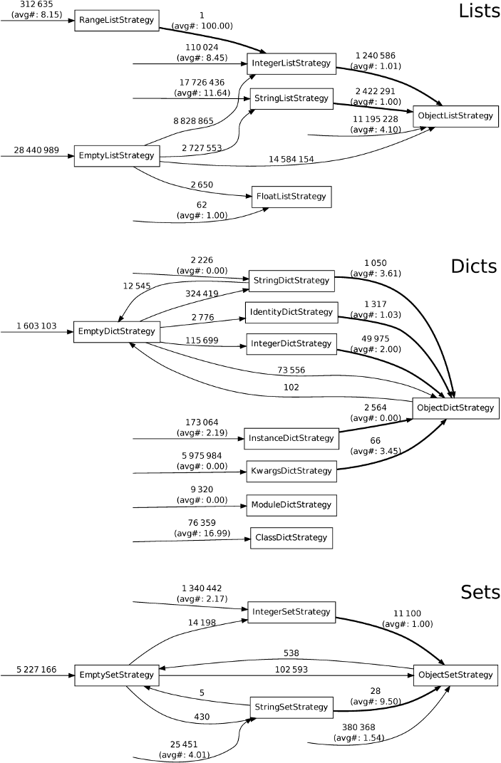
In Section 3, we stated two hypotheses about real-world programs, which led us to create storage strategies as they are. We can also slightly narrow the scope of interest for the hypotheses to ints, floats, and strings, as these are the only cases which affect storage strategies. Usefully, storage strategies themselves give us a simple way of validating the hypotheses. We created a PyPy variant with two counters for each storage strategy, recording the number of times a transition from one storage strategy to another is taken, and the size of the collection at that point, allowing us to trivially calculate the average size of a collection’s elements at switch. Figure 6 shows the resulting cumulative transition diagram for the real-world benchmarks from Table 1.
Hypothesis H1 postulates that “it is uncommon for a homogeneously typed collection storing objects of primitive types to later have an element of a different type added to it.” The basis for this hypothesis is our expectation that, even in dynamically typed languages, programmers often use collections in a type homogeneous fashion. Figure 6 clearly shows this. The transitions of interest are those where elements are either created or reboxed (shown in bold), which is where the hypothesis is violated. Consider StringListStrategy, which is the biggest example. Around 21 million lists are created with that storage strategy, but only a little over 15% type dehomogenise. On average, across the whole of Figure 6, a little under 10% of collections using optimised storage strategies later type dehomogenise. Some benchmarks (e.g. Feedparser and orm) type dehomogenise more than double this amount of objects: both see little gain from storage strategies. As this suggests, programs which violate hypothesis H1 may perform worse with storage strategies than without.
Hypothesis H2 postulates that “when a previously homogeneously typed collection type dehomogenises, the transition happens after only a small number of elements have been added.” The basis for this hypothesis follows from H1, and is our expectation that when a collection does type dehomogenise, it contains few elements. Therefore, we are really interested in how often the ‘worst case’ scenario – extremely large collections type dehomogenising – happens. A sensible measure is thus the average number of elements a collection contains when type dehomogenisation occurs. As Figure 6 shows, when collections using optimised storage strategies type dehomogenise, they typically contain only a single element. The costs of such a switch are, thus, minimal.
We consider the evidence for hypothesis H1 strong and that for H2 conclusive. The validation of these hypotheses also goes some way to explain why storage strategies are effective: although the potential worst case is deeply unpleasant, programmers do not write programs which run in a way that triggers the worst case.
5.7 Threats to validity
For the speed benchmarks, the main threat to validity is that we report performance in PyPy’s steady-state, largely excluding start-up times. While this is representative of a large class of programs – e.g. server programs, or those which perform long calculations – it does not tend to represent short-lived batch-like programs very well. Balancing these two factors is a perennial problem when measuring the performance of programs in JIT VMs, because the ‘best’ answer is highly dependent on how an individual user uses the JIT. The virtue of using steady-state measurements for this paper is that the numbers are more stable: measuring numbers before the steady-state is reached can be highly volatile, as the impact of the JIT can be significant.
For the memory benchmarks, a significant threat to validity is that we manually chose the locations in the program to measure peak memory usage. We may unwittingly have chosen locations which favour storage strategies. However, by using large number of benchmarks, we have reduced the chances of this potential bias having a significant effect.
6. Relevance to other languages
The evaluation in Section 5 shows that enough real-world Python programs’ collections contain elements of a single primitive type to make storage strategies a substantial optimisation. We now consider an important question: are storage strategies only relevant to Python (the language) or PyPy (the language implementation)?
Perhaps the most important results in the evaluation are the statistic surrounding type dehomogenisation (Section 5.6) which show that: collections of primitive types dehomogenise in only 10% of cases; when type dehomogenisation occurs, collections only contain a single element on average. These two statistics go a considerable way to explain why storage strategies are so effective. We believe that programs in most dynamically typed languages will follow a similar pattern, for the simple reason that this is the most predictable, safe way to develop programs. We therefore expect that most dynamically typed language implementations have the same underlying potential for improvement that we have shown with PyPy.
Importantly, we do not believe that storage strategies only make sense when used in the lowest-level VM: language implementations running atop an existing VM can easily use storage strategies. For example, an implementation such as Jython (Python running on the JVM) could make use of storage strategies. We do, however, note that JIT-based implementations seem likely to see larger relative benefits from storage strategies than non-JIT-based implementations because of the ability of the JIT to more frequently unbox elements. However, this should apply equally well to language implementations running atop another JIT-based VM.
7. Related Work
Pointer tagging is the obvious ‘alternative’ to storage strategies (see Section 2.1). There is currently no direct comparison between pointer tagging and storage strategies. It is therefore possible that pointer tagging could provide a more efficient solution to storing easily tagged items such as integers or floats. However, as Table 3 clearly shows, a significant part of the speed-up of storage strategies comes from strings. On a 64-bit machine, 7 bytes in a tagged pointer could be used for strings; strings longer than that would have to be allocated on the heap. To get an idea of how often large strings are used, we created a PyPy variant (included in our downloadable experiment) to count the length of every string allocated in the benchmark suite from Section 5. 64% of the strings created by our benchmark suite from Section 5 are larger than 7 bytes (85% are bigger than 3 bytes, the cut-off point for 32-bit machines). We caution against over-interpreting these numbers. First, we can not easily separate out strings used internally by PyPy’s interpreter. However such strings are, by design, small, so the numbers we obtained are lower-bounds for the real numbers of strings too large to be used with tagging. Second, we suspect that the length of strings used by different programs varies more than many other factors. Nevertheless, these numbers indicate that storage strategies can outperform pointer tagging.
The inspiration behind storage strategies is the map concept, which originated in the Self project as a way to efficiently represent prototype objects with varying sets of instance field names [11 ]. This is done by splitting objects into a (mostly constant) map and a (continually changing) storage area. The map describes where within the storage area slot names can be looked up. Maps have two benefits. When using an interpreter or a JIT, they lower memory consumption (since maps are shared between objects, with only the storage area being unique to each object). When the JIT is used, they also significantly speed-up slot lookups because the constant nature of maps allows JITs to fold away many computations based upon them. Storage strategies similarly split apart a collection and its data; some optimised storage strategies also identify some data as being constant in a similar way to maps, though not all strategies are able to do so.
The only other VM we are aware of which uses a mechanism comparable to storage strategies is V8 [13, 14]. Arrays are specialised with an ‘element kind’ which determines the memory layout, in similar fashion to storage strategies. Unlike PyPy, in V8 an array’s default storage strategy is equivalent to what we might call IntegerArrayStrategy. If a float is added to an array with IntegerArrayStrategy, the storage strategy is changed to FloatArrayStrategy and the storage area revised accordingly. Non-numeric objects added to arrays with IntegerArrayStrategy or FloatArrayStrategy cause a transition to ObjectArrayStrategy, forcing existing elements to be reboxed. Emptying a V8 array does not reset its element kind, which thus moves monotonically towards ObjectArrayStrategy.
To avoid strategy changes, array creation sites in a program can create arrays with different initial strategies. To do this, arrays can track from which part of the program they were created. When an array’s storage strategy changes, the site which created it is informed. Subsequent arrays created from that site are initialised with the revised storage strategy (though existing arrays are left as-is), even if those subsequent arrays will never change strategy. V8’s element kinds thus aim to minimise type dehomogenisation, while PyPy’s storage strategies attempt to optimise every possible collection. To understand how these two schemes work in practise, we created a PyPy variant (included in our downloadable experiment) to see how often collections of one specific creation site type dehomogenise. 98.8% of the collection creation sites do not type dehomogenise at all. Of those which do type dehomogenise, around one third always create collections that all dehomogenise. The remaining two thirds of sites create some collections which dehomogenise and some which do not; the distribution has no clear pattern and we are currently unable to determine the size of the collections involved.
V8 has several mechanisms to mitigate the likelihood of array creation sites unnecessarily being set to ObjectArrayStrategy (which is particularly likely for e.g. factory functions). Notably, when a function is compiled by the JIT compiler, array call sites become fixed and any changes of strategy to arrays created from those sites are ignored. A deoptimisation has to occur before those call sites’ element kinds can be reconsidered.
Overall, it is unclear what the performance implications of V8 and PyPy’s approaches are: both have troubling worst-case performance, but neither situation appears to happen often in real programs. We suspect that each approach will perform similarly due to the typical nature of dynamically typed programs (see Section 5.6).
While storage strategies and V8’s kinds are fully dynamic, Hackett and Guo show how a type inferencer for Java can optimise many arrays [22]. The unsound type inferencer is combined with dynamic type checks to make a reliable system: type assumptions are adjusted as and when the program violates them. Similarly to V8, array types are referenced from each creation site. While, in Javascript, this may well result in similar, or better, performance to V8’s kinds, its relevance to Python is unclear. Python programs frequently frustrate type inferencers [10], which may only allow small improvements in collections performance.
There has been substantial work on memory optimisation in the JVM, though most of it is orthogonal to storage strategies, perhaps reflecting the work’s origins in optimising embedded systems. [34] details various memory inefficiencies found from a series of Java benchmarks, before describing how previously published approaches (e.g. object sharing [2] and data compression [1 ]) may be able to address them. Such techniques can potentially be applied alongside storage strategies, though it is unclear if the real-world benefits would justify the effort involved in doing so.
8. Conclusions
Storage strategies are a simple technique for improving the performance of real-world dynamically typed languages and which we believe has wide applicability. We suspect that the core storage strategies presented in this paper (particularly lists and dictionaries, integers and strings) will be applicable to virtually every dynamically typed language and its implementations. However, different language’s semantics and idioms of use may mean that different ‘exotic’ storage strategies are needed relative to those in PyPy.
Storage strategies also make it feasible to experiment with more exotic techniques such as data compression, and could also allow user-level code to determine storage layout (in similar spirit to CLOS). It may also be possible to reuse parts of existing strategies when implementing new collection types.
An important avenue for future research will be to reduce storage strategies’ worst case behaviour (when type dehomogenising collections using specialised storage strategies). It is possible that a hybrid of V8’s kinds (which take into account a collection’s creation site) and storage strategies may allow a scheme to be created which avoids the worst case performance of each.
Acknowledgments
We thank: Michael Leuschel, David Schneider, Samuele Pedroni, Sven Hager, and Michael Perscheid for insightful comments on various drafts of the paper; and Daniel Clifford, Vyacheslav Egorov, and Michael Stanton for providing insight on V8’s mechanism. This research was partly funded by the EPSRC Cooler grant EP/K01790X/1.
References
[1] C. S. Ananian and M. Rinard. Data size optimizations for Java programs. In Proc. LCTES, pages 59–68, 2003.
[2] A. W. Appel and M. J. Gonçalves. Hash-consing garbage collection. Technical Report CS-TR-412-93, Princeton University, Dept. of Computer Science, 1993.
[3] V. Bala, E. Duesterwald, and S. Banerjia. Dynamo: a transparent dynamic optimization system. In Proc. PLDI, pages 1–12, 2000.
[4] M. Bayer. Orm2010, 2012. URL http://techspot.zzzeek.org. [Online; accessed 26-March-2013].
[5] S. Bird, E. Klein, and E. Loper. Natural Language Processing with Python. O’Reilly Media, July 2009.
[6] C. F. Bolz and L. Tratt. The impact of meta-tracing on VM design and implementation. To appear, Science of Computer Programming, 2013.
[7] C. F. Bolz, A. Cuni, M. Fijałkowski, and A. Rigo. Tracing the meta-level: PyPy’s tracing JIT compiler. In Proc. ICOOOLPS, pages 18–25, 2009.
[8] C. F. Bolz, A. Cuni, M. Fijałkowski, M. Leuschel, S. Pedroni, and A. Rigo. Allocation removal by partial evaluation in a tracing JIT. Proc. PEPM, Jan. 2011.
[9] O. Callaú, R. Robbes, E. Tanter, and D. Röthlisberger. How developers use the dynamic features of programming languages: the case of smalltalk. In Proc. MSR, page 23–32, 2011.
[10] B. Cannon. Localized type inference of atomic types in Python. Master thesis, California Polytechnic State University, 2005.
[11] C. Chambers, D. Ungar, and E. Lee. An efficient implementation of SELF a dynamically-typed object-oriented language based on prototypes. In OOPSLA, volume 24, 1989.
[12] C. Chambers, D. Ungar, and E. Lee. An efficient implementation of self a dynamically-typed object-oriented language based on prototypes. SIGPLAN Not., 24:49–70, Sept. 1989.
[13] D. Clifford. URL http://v8-io12.appspot.com/. Talk at IO12 [Online; accessed 27-June-2013].
[14] D. Clifford, V. Egorov, and M. Stanton. Personal communication, July 2013.
[15] J. da Silva and G. Lopes. A local maxima method and a fair dispersion normalization for extracting multi-word units from corpora. In Meeting on Mathematics of Language, 1999.
[16] FeedParser Developers. Feedparser, 2012. URL http://code.google.com/p/feedparser/. [Online; accessed 26-March-2013].
[17] P. Fleming and J. Wallace. How not to lie with statistics: the correct way to summarize benchmark results. Commun. ACM, 29(3):218–221, Mar. 1986.
[18] A. Gal, B. Eich, M. Shaver, D. Anderson, D. Mandelin, M. R. Haghighat, B. Kaplan, G. Hoare, B. Zbarsky, J. Orendorff, J. Ruderman, E. W. Smith, R. Reitmaier, M. Bebenita, M. Chang, and M. Franz. Trace-based Just-In-Time type specialization for dynamic languages. In Proc. PLDI, 2009.
[19] E. Gamma, R. Helm, R. E. Johnson, and J. Vlissides. Design Patterns: Elements of Reusable Object-Oriented Software. Addison-Wesley Longman, Amsterdam, Oct. 1994.
[20] A. Georges, D. Buytaert, and L. Eeckhout. Statistically rigorous Java performance evaluation. SIGPLAN Notices, 42 (10):57–76, 2007.
[21] D. Gudeman. Representing type information in Dynamically-Typed languages. Technical Report TR93-27, University of Arizona at Tucson, 1993.
[22] B. Hackett and S.-y. Guo. Fast and precise hybrid type inference for JavaScript. In Proc. PLDI, pages 239–250, 2012.
[23] A. Holkner and J. Harland. Evaluating the dynamic behaviour of python applications. In Proc. ACSC, pages 19–28, 2009.
[24] T. Kotzmann and H. Mössenböck. Escape analysis in the context of dynamic compilation and deoptimization. In Proc. VEE, page 111–120, 2005.
[25] Logilab. Pylint, 2012. URL http://www.logilab.org/project/pylint. [Online; accessed 26-March-2013].
[26] NetworkX Developers. Networkx, 2012. URL http://networkx.lanl.gov. [Online; accessed 26-March-2013].
[27] pyExcelerator Developers. pyexcelerator, 2012. URL http://sourceforge.net/projects/pyexcelerator. [Online; accessed 26-March-2013].
[28] PyPy Team. Pypy speed benchmarks, 2013. URL http://speed.pypy.org/. [Online; accessed 27-June-2013].
[29] P. Quentel. Pydblite, 2012. URL http://www.pydblite.net/en/index.html. [Online; accessed 26-March-2013].
[30] A. Radziszewski and M. Piasecki. A preliminary Noun Phrase Chunker for Polish. In Proc. IOS, pages 169–180. Springer, 2010. Chunker available at http://nlp.pwr.wroc.pl/trac/private/disaster/.
[31] G. Richards, S. Lebresne, B. Burg, and J. Vitek. An analysis of the dynamic behavior of JavaScript programs. In Proc. PLDI, pages 1–12, 2010.
[32] A. Rigo and S. Pedroni. PyPy’s approach to virtual machine construction. In Proc. DLS, 2006.
[33] Rosetta Code. Inverted index, 2012. URL http://rosettacode.org/wiki/Inverted_index#Python. [Online; accessed 26-March-2013].
[34] J. B. Sartor, M. Hirzel, and K. S. McKinley. No bit left behind: the limits of heap data compression. In Proc. ISSM, pages 111–120. ACM, 2008.
[35] L. Tratt. Dynamically typed languages. Advances in Computers, 77:149–184, July 2009.
[36] Whoosh Developers. Whoosh, 2012. URL https://bitbucket.org/mchaput/whoosh. [Online; accessed 26-March-2013].
A. Appendix
| Benchmark | pypy-none | pypy-all | pypy-list | pypy-set | pypy-dict | pypy-ints | pypy-strings | pypy-floats
| ||||||||||||||||
| disaster | 14.219 | ± | 0.206 | 13.357 | ± | 0.223 | 14.651 | ± | 0.201 | 13.496 | ± | 0.186 | 13.743 | ± | 0.210 | 13.403 | ± | 0.181 | 13.241 | ± | 0.200 | 13.254 | ± | 0.134 |
| Feedparser | 0.801 | ± | 0.258 | 0.800 | ± | 0.265 | 0.799 | ± | 0.263 | 0.800 | ± | 0.231 | 0.797 | ± | 0.257 | 0.803 | ± | 0.265 | 0.803 | ± | 0.256 | 0.798 | ± | 0.243 |
| invindex | 20.643 | ± | 0.167 | 2.808 | ± | 0.042 | 2.797 | ± | 0.010 | 23.774 | ± | 0.112 | 24.199 | ± | 0.056 | 23.607 | ± | 0.067 | 2.826 | ± | 0.015 | 24.842 | ± | 0.131 |
| multiwords | 1.293 | ± | 0.015 | 1.238 | ± | 0.016 | 1.233 | ± | 0.015 | 1.256 | ± | 0.013 | 1.285 | ± | 0.016 | 1.279 | ± | 0.037 | 1.339 | ± | 0.046 | 1.311 | ± | 0.054 |
| NetworkX | 2.383 | ± | 0.054 | 1.387 | ± | 0.015 | 2.274 | ± | 0.009 | 2.489 | ± | 0.016 | 1.486 | ± | 0.010 | 1.338 | ± | 0.014 | 1.759 | ± | 0.017 | 1.865 | ± | 0.029 |
| nltk-wordassoc | 1.160 | ± | 0.015 | 1.077 | ± | 0.014 | 1.100 | ± | 0.012 | 1.171 | ± | 0.014 | 1.142 | ± | 0.011 | 1.177 | ± | 0.013 | 1.062 | ± | 0.014 | 1.180 | ± | 0.015 |
| orm | 24.584 | ± | 2.057 | 24.330 | ± | 1.953 | 24.542 | ± | 2.066 | 24.531 | ± | 1.986 | 24.006 | ± | 2.059 | 24.265 | ± | 2.179 | 23.866 | ± | 2.134 | 24.712 | ± | 2.099 |
| PyDbLite | 0.221 | ± | 0.003 | 0.196 | ± | 0.003 | 0.227 | ± | 0.002 | 0.230 | ± | 0.001 | 0.193 | ± | 0.001 | 0.253 | ± | 0.001 | 0.196 | ± | 0.001 | 0.252 | ± | 0.001 |
| PyExcelerator | 12.106 | ± | 0.048 | 11.932 | ± | 0.029 | 12.797 | ± | 0.045 | 11.862 | ± | 0.046 | 11.427 | ± | 0.027 | 12.293 | ± | 0.033 | 11.571 | ± | 0.030 | 12.037 | ± | 0.025 |
| Scapy | 0.202 | ± | 0.031 | 0.136 | ± | 0.026 | 0.202 | ± | 0.030 | 0.204 | ± | 0.031 | 0.137 | ± | 0.026 | 0.170 | ± | 0.035 | 0.141 | ± | 0.026 | 0.174 | ± | 0.036 |
| slowsets | 38.333 | ± | 0.122 | 33.777 | ± | 0.838 | 39.027 | ± | 1.073 | 34.767 | ± | 1.607 | 38.669 | ± | 0.091 | 37.750 | ± | 0.231 | 34.249 | ± | 0.844 | 37.831 | ± | 0.096 |
| whoosh | 1.435 | ± | 0.014 | 1.313 | ± | 0.015 | 1.395 | ± | 0.014 | 1.416 | ± | 0.015 | 1.291 | ± | 0.020 | 1.387 | ± | 0.015 | 1.278 | ± | 0.014 | 1.401 | ± | 0.012 |
| ai | 0.064 | ± | 0.003 | 0.048 | ± | 0.004 | 0.055 | ± | 0.003 | 0.054 | ± | 0.003 | 0.060 | ± | 0.003 | 0.047 | ± | 0.003 | 0.067 | ± | 0.003 | 0.056 | ± | 0.003 |
| bm_chameleon | 0.017 | ± | 0.000 | 0.015 | ± | 0.000 | 0.017 | ± | 0.000 | 0.016 | ± | 0.000 | 0.015 | ± | 0.000 | 0.017 | ± | 0.000 | 0.016 | ± | 0.000 | 0.016 | ± | 0.000 |
| bm_mako | 0.030 | ± | 0.014 | 0.029 | ± | 0.013 | 0.031 | ± | 0.014 | 0.031 | ± | 0.014 | 0.030 | ± | 0.013 | 0.030 | ± | 0.013 | 0.031 | ± | 0.013 | 0.031 | ± | 0.014 |
| chaos | 0.020 | ± | 0.001 | 0.008 | ± | 0.000 | 0.008 | ± | 0.000 | 0.016 | ± | 0.000 | 0.016 | ± | 0.000 | 0.008 | ± | 0.000 | 0.020 | ± | 0.000 | 0.021 | ± | 0.000 |
| crypto_pyaes | 0.055 | ± | 0.002 | 0.054 | ± | 0.002 | 0.054 | ± | 0.002 | 0.054 | ± | 0.002 | 0.053 | ± | 0.002 | 0.053 | ± | 0.002 | 0.054 | ± | 0.002 | 0.054 | ± | 0.002 |
| django | 0.051 | ± | 0.000 | 0.037 | ± | 0.000 | 0.047 | ± | 0.000 | 0.051 | ± | 0.000 | 0.040 | ± | 0.000 | 0.044 | ± | 0.000 | 0.036 | ± | 0.000 | 0.044 | ± | 0.000 |
| fannkuch | 0.148 | ± | 0.001 | 0.142 | ± | 0.000 | 0.143 | ± | 0.001 | 0.171 | ± | 0.001 | 0.168 | ± | 0.001 | 0.143 | ± | 0.001 | 0.179 | ± | 0.001 | 0.158 | ± | 0.001 |
| genshi_text | 0.022 | ± | 0.002 | 0.019 | ± | 0.001 | 0.022 | ± | 0.001 | 0.024 | ± | 0.002 | 0.019 | ± | 0.001 | 0.023 | ± | 0.001 | 0.019 | ± | 0.001 | 0.022 | ± | 0.002 |
| go | 0.098 | ± | 0.037 | 0.092 | ± | 0.037 | 0.095 | ± | 0.038 | 0.098 | ± | 0.037 | 0.098 | ± | 0.037 | 0.092 | ± | 0.037 | 0.100 | ± | 0.037 | 0.099 | ± | 0.037 |
| html5lib | 2.626 | ± | 0.058 | 2.426 | ± | 0.042 | 2.466 | ± | 0.054 | 2.682 | ± | 0.055 | 2.508 | ± | 0.056 | 2.449 | ± | 0.039 | 2.405 | ± | 0.041 | 2.454 | ± | 0.038 |
| meteor-contest | 0.154 | ± | 0.002 | 0.099 | ± | 0.002 | 0.156 | ± | 0.002 | 0.097 | ± | 0.001 | 0.155 | ± | 0.001 | 0.100 | ± | 0.002 | 0.145 | ± | 0.002 | 0.104 | ± | 0.002 |
| nbody_modified | 0.035 | ± | 0.000 | 0.035 | ± | 0.000 | 0.032 | ± | 0.000 | 0.033 | ± | 0.002 | 0.033 | ± | 0.000 | 0.033 | ± | 0.000 | 0.033 | ± | 0.000 | 0.033 | ± | 0.000 |
| pyflate-fast | 0.381 | ± | 0.008 | 0.324 | ± | 0.008 | 0.331 | ± | 0.009 | 0.388 | ± | 0.017 | 0.391 | ± | 0.018 | 0.358 | ± | 0.007 | 0.347 | ± | 0.013 | 0.381 | ± | 0.008 |
| raytrace-simple | 0.024 | ± | 0.004 | 0.024 | ± | 0.006 | 0.025 | ± | 0.005 | 0.026 | ± | 0.005 | 0.025 | ± | 0.005 | 0.024 | ± | 0.004 | 0.024 | ± | 0.004 | 0.025 | ± | 0.007 |
| richards | 0.004 | ± | 0.000 | 0.004 | ± | 0.000 | 0.004 | ± | 0.000 | 0.004 | ± | 0.000 | 0.004 | ± | 0.000 | 0.004 | ± | 0.000 | 0.004 | ± | 0.001 | 0.004 | ± | 0.000 |
| slowspitfire | 0.275 | ± | 0.004 | 0.250 | ± | 0.002 | 0.227 | ± | 0.009 | 0.270 | ± | 0.007 | 0.271 | ± | 0.008 | 0.275 | ± | 0.012 | 0.250 | ± | 0.020 | 0.284 | ± | 0.013 |
| spambayes | 0.085 | ± | 0.047 | 0.081 | ± | 0.044 | 0.083 | ± | 0.046 | 0.086 | ± | 0.045 | 0.082 | ± | 0.043 | 0.082 | ± | 0.046 | 0.082 | ± | 0.043 | 0.083 | ± | 0.046 |
| spectral-norm | 0.014 | ± | 0.001 | 0.014 | ± | 0.001 | 0.014 | ± | 0.001 | 0.014 | ± | 0.001 | 0.014 | ± | 0.001 | 0.014 | ± | 0.001 | 0.014 | ± | 0.001 | 0.014 | ± | 0.001 |
| sympy_integrate | 0.872 | ± | 0.218 | 0.815 | ± | 0.152 | 0.887 | ± | 0.214 | 0.868 | ± | 0.222 | 0.849 | ± | 0.208 | 0.884 | ± | 0.204 | 0.839 | ± | 0.148 | 0.876 | ± | 0.208 |
| telco | 0.045 | ± | 0.006 | 0.039 | ± | 0.007 | 0.041 | ± | 0.007 | 0.043 | ± | 0.007 | 0.039 | ± | 0.008 | 0.039 | ± | 0.006 | 0.039 | ± | 0.008 | 0.041 | ± | 0.006 |
| twisted_names | 0.002 | ± | 0.000 | 0.002 | ± | 0.000 | 0.002 | ± | 0.000 | 0.002 | ± | 0.000 | 0.002 | ± | 0.000 | 0.002 | ± | 0.000 | 0.002 | ± | 0.000 | 0.002 | ± | 0.000 |
| Benchmark | pypy-all | pypy-list | pypy-ints
| ||||||
| | * pypy-dict | * pypy-strings
| |||||||
| | * pypy-set | * pypy-floats
| |||||||
| disaster | 0.939 | ± | 0.021 | 0.945 | ± | 0.033 = | 0.818 | ± | 0.028 < |
| Feedparser | 0.999 | ± | 0.461 | 0.991 | ± | 0.771 = | 1.002 | ± | 0.785 = |
| invindex | 0.136 | ± | 0.002 | 0.183 | ± | 0.003 > | 0.188 | ± | 0.003 > |
| multiwords | 0.958 | ± | 0.016 | 0.921 | ± | 0.026 = | 1.038 | ± | 0.066 = |
| NetworkX | 0.582 | ± | 0.015 | 0.621 | ± | 0.025 = | 0.324 | ± | 0.014 < |
| nltk-wordassoc | 0.928 | ± | 0.017 | 0.942 | ± | 0.028 = | 0.944 | ± | 0.029 = |
| orm | 0.990 | ± | 0.115 | 0.973 | ± | 0.199 = | 0.963 | ± | 0.203 = |
| PyDbLite | 0.888 | ± | 0.017 | 0.939 | ± | 0.022 > | 1.169 | ± | 0.025 > |
| PyExcelerator | 0.986 | ± | 0.005 | 0.978 | ± | 0.009 = | 0.965 | ± | 0.008 < |
| Scapy | 0.671 | ± | 0.164 | 0.680 | ± | 0.264 = | 0.503 | ± | 0.220 = |
| slowsets | 0.881 | ± | 0.022 | 0.931 | ± | 0.050 = | 0.868 | ± | 0.023 = |
| whoosh | 0.915 | ± | 0.014 | 0.863 | ± | 0.023 < | 0.840 | ± | 0.020 < |
| ai | 0.748 | ± | 0.068 | 0.694 | ± | 0.090 = | 0.686 | ± | 0.088 = |
| bm_chameleon | 0.893 | ± | 0.009 | 0.761 | ± | 0.008 < | 0.838 | ± | 0.007 < |
| bm_mako | 0.956 | ± | 0.615 | 1.097 | ± | 1.211 = | 1.087 | ± | 1.202 = |
| chaos | 0.403 | ± | 0.011 | 0.246 | ± | 0.012 < | 0.430 | ± | 0.021 = |
| crypto_pyaes | 0.985 | ± | 0.050 | 0.944 | ± | 0.082 = | 0.940 | ± | 0.083 = |
| django | 0.721 | ± | 0.011 | 0.747 | ± | 0.017 = | 0.541 | ± | 0.014 < |
| fannkuch | 0.956 | ± | 0.005 | 1.266 | ± | 0.013 > | 1.252 | ± | 0.012 > |
| genshi_text | 0.871 | ± | 0.086 | 0.933 | ± | 0.157 = | 0.933 | ± | 0.158 = |
| go | 0.940 | ± | 0.517 | 0.961 | ± | 0.894 = | 0.959 | ± | 0.887 = |
| html5lib | 0.924 | ± | 0.026 | 0.915 | ± | 0.049 = | 0.798 | ± | 0.038 < |
| meteor-contest | 0.645 | ± | 0.017 | 0.651 | ± | 0.022 = | 0.415 | ± | 0.017 < |
| nbody_modified | 0.986 | ± | 0.007 | 0.810 | ± | 0.061 < | 0.821 | ± | 0.011 < |
| pyflate-fast | 0.850 | ± | 0.027 | 0.906 | ± | 0.072 = | 0.856 | ± | 0.052 = |
| raytrace-simple | 0.990 | ± | 0.291 | 1.161 | ± | 0.552 = | 1.050 | ± | 0.522 = |
| richards | 0.882 | ± | 0.066 | 0.815 | ± | 0.103 = | 0.834 | ± | 0.266 = |
| slowspitfire | 0.908 | ± | 0.014 | 0.797 | ± | 0.049 < | 0.938 | ± | 0.099 = |
| spambayes | 0.956 | ± | 0.743 | 0.967 | ± | 1.290 = | 0.924 | ± | 1.247 = |
| spectral-norm | 0.993 | ± | 0.137 | 0.993 | ± | 0.239 = | 0.980 | ± | 0.234 = |
| sympy_integrate | 0.935 | ± | 0.291 | 0.987 | ± | 0.601 = | 0.981 | ± | 0.561 = |
| telco | 0.858 | ± | 0.185 | 0.741 | ± | 0.274 = | 0.672 | ± | 0.233 = |
| twisted_names | 0.921 | ± | 0.032 | 0.915 | ± | 0.052 = | 0.897 | ± | 0.052 = |
| Combined Ratios | 0.816 | ± | 0.034 | 0.813 | ± | 0.058 = | 0.783 | ± | 0.057 = |